29  Modeling with k-means clustering - diab_pop

29.1 SET UP

library(tidyverse)

── Attaching core tidyverse packages ──────────────────────── tidyverse 2.0.0 ──
✔ dplyr     1.2.1     ✔ readr     2.2.0
✔ forcats   1.0.1     ✔ stringr   1.6.0
✔ ggplot2   4.0.3     ✔ tibble    3.3.1
✔ lubridate 1.9.5     ✔ tidyr     1.3.2
✔ purrr     1.2.2     
── Conflicts ────────────────────────────────────────── tidyverse_conflicts() ──
✖ dplyr::filter() masks stats::filter()
✖ dplyr::lag()    masks stats::lag()
ℹ Use the conflicted package (<http://conflicted.r-lib.org/>) to force all conflicts to become errors

library(factoextra)

Welcome to factoextra!
Want to learn more? See two factoextra-related books at https://www.datanovia.com/en/product/practical-guide-to-principal-component-methods-in-r/

library('caret')

Loading required package: lattice

Attaching package: 'caret'

The following object is masked from 'package:purrr':

    lift

diab_pop <- readRDS(here::here('DATA/diab_pop.RDS')) %>%
  na.omit() 

numeric_features <- diab_pop %>%
  select_if(is.numeric) %>%
  select(-seqn) %>%
  colnames()

29.2 Split Data

TrainInd <- createDataPartition(diab_pop$diq010,
                                p=.7,
                                list=FALSE)

TRAIN <- diab_pop[TrainInd,]

29.2.1 How many Clusters should we make ?

fviz_nbclust(TRAIN %>%
               select(numeric_features) %>%
               scale(),
              kmeans, 
              method='wss')

Warning: Using an external vector in selections was deprecated in tidyselect 1.1.0.
ℹ Please use `all_of()` or `any_of()` instead.
  # Was:
  data %>% select(numeric_features)

  # Now:
  data %>% select(all_of(numeric_features))

See <https://tidyselect.r-lib.org/reference/faq-external-vector.html>.

29.3 Train Clustering Model

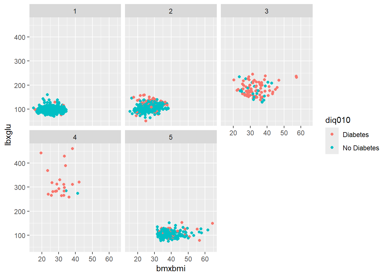
# Set seed for reproducible results
set.seed(1984)


pP.TRAIN <- preProcess(TRAIN, c('center','scale'))

# Run k-means algorithm
# Nstart = # random starting positions; I chose 523
km <- kmeans(predict(pP.TRAIN, TRAIN) %>% select(numeric_features), 
             centers = 5, 
             nstart = 523)

glimpse(km)

List of 9
 $ cluster     : Named int [1:1314] 1 1 4 2 4 3 3 2 4 4 ...
  ..- attr(*, "names")= chr [1:1314] "2" "3" "11" "15" ...
 $ centers     : num [1:5, 1:3] 0.894 0.254 0.833 -0.893 -0.735 ...
  ..- attr(*, "dimnames")=List of 2
  .. ..$ : chr [1:5] "1" "2" "3" "4" ...
  .. ..$ : chr [1:3] "ridageyr" "bmxbmi" "lbxglu"
 $ totss       : num 3939
 $ withinss    : num [1:5] 317 172 273 264 208
 $ tot.withinss: num 1234
 $ betweenss   : num 2705
 $ size        : int [1:5] 437 44 179 444 210
 $ iter        : int 4
 $ ifault      : int 0
 - attr(*, "class")= chr "kmeans"

TRAIN.cluster <- cbind(TRAIN, cluster=km$cluster)

head(TRAIN.cluster)

    seqn riagendr ridageyr           ridreth1                 dmdeduc2
2  83733     Male       53 Non-Hispanic White High school graduate/GED
3  83734     Male       78 Non-Hispanic White High school graduate/GED
11 83750     Male       45              Other            Grades 9-11th
15 83757   Female       57     Other Hispanic      Less than 9th grade
17 83761   Female       24              Other    College grad or above
29 83787   Female       68    MexicanAmerican      Less than 9th grade
        dmdmartl        indhhin2 bmxbmi      diq010 lbxglu cluster
2       Divorced $15,000-$19,999   30.8 No Diabetes    101       1
3        Married $20,000-$24,999   28.8    Diabetes     84       1
11 Never married $65,000-$74,999   24.1 No Diabetes     84       4
15     Separated $20,000-$24,999   35.4    Diabetes    398       2
17 Never married       $0-$4,999   25.3 No Diabetes     95       4
29      Divorced $15,000-$19,999   33.5 No Diabetes    111       3

fviz_cluster(km, 
             data = TRAIN.cluster %>%
               select(numeric_features, cluster) %>%
               scale()
             )

km$centers

    ridageyr     bmxbmi     lbxglu
1  0.8939479 -0.4320271 -0.1059434
2  0.2544713  0.1864569  4.3200213
3  0.8325803  1.2355374  0.4141108
4 -0.8931606 -0.6454971 -0.3694405
5 -0.7348597  1.1715773 -0.2565617

library(ggplot2)

TRAIN.cluster <- TRAIN.cluster %>%
  mutate(cluster= as.factor(cluster))

TRAIN.cluster %>%
  ggplot(aes(x=ridageyr,
             y=lbxglu,
             color=cluster)) +
  geom_point()

Plot_Clusters_by_Facet = function(dat, x, y, c, z) {
     ggplot(dat, 
            aes(x = .data[[x]], 
                y = .data[[y]],
                color=.data[[c]])
            ) +
          geom_point() +
          facet_wrap(.data[[z]] ~ .)
}


Plot_Clusters_by_Facet(TRAIN.cluster, 
            x='ridageyr',
            y='lbxglu',
            c='cluster',
            z='diq010')

Plot_Clusters_by_Facet(TRAIN.cluster, 
            x='bmxbmi',
            y='lbxglu',
            c='diq010',
            z='cluster')

library('arsenal')

Attaching package: 'arsenal'

The following object is masked from 'package:lubridate':

    is.Date

library('knitr')
library('kableExtra')

Attaching package: 'kableExtra'

The following object is masked from 'package:dplyr':

    group_rows

table_arsenal <- tableby(diq010 ~ cluster , 
                         data = TRAIN.cluster)

table_arsenal

tableby Object

Function Call:
tableby(formula = diq010 ~ cluster, data = TRAIN.cluster)

Variable(s):
diq010 ~ cluster

summary(table_arsenal)

|                    | Diabetes (N=197) | No Diabetes (N=1117) | Total (N=1314) | p value|
|:-------------------|:----------------:|:--------------------:|:--------------:|-------:|
|**cluster**         |                  |                      |                | < 0.001|
|&nbsp;&nbsp;&nbsp;1 |    76 (38.6%)    |     361 (32.3%)      |  437 (33.3%)   |        |
|&nbsp;&nbsp;&nbsp;2 |    39 (19.8%)    |       5 (0.4%)       |   44 (3.3%)    |        |
|&nbsp;&nbsp;&nbsp;3 |    63 (32.0%)    |     116 (10.4%)      |  179 (13.6%)   |        |
|&nbsp;&nbsp;&nbsp;4 |     7 (3.6%)     |     437 (39.1%)      |  444 (33.8%)   |        |
|&nbsp;&nbsp;&nbsp;5 |    12 (6.1%)     |     198 (17.7%)      |  210 (16.0%)   |        |

sum.table_arsenal <- summary(table_arsenal)

sum.table_arsenal

|                    | Diabetes (N=197) | No Diabetes (N=1117) | Total (N=1314) | p value|
|:-------------------|:----------------:|:--------------------:|:--------------:|-------:|
|**cluster**         |                  |                      |                | < 0.001|
|&nbsp;&nbsp;&nbsp;1 |    76 (38.6%)    |     361 (32.3%)      |  437 (33.3%)   |        |
|&nbsp;&nbsp;&nbsp;2 |    39 (19.8%)    |       5 (0.4%)       |   44 (3.3%)    |        |
|&nbsp;&nbsp;&nbsp;3 |    63 (32.0%)    |     116 (10.4%)      |  179 (13.6%)   |        |
|&nbsp;&nbsp;&nbsp;4 |     7 (3.6%)     |     437 (39.1%)      |  444 (33.8%)   |        |
|&nbsp;&nbsp;&nbsp;5 |    12 (6.1%)     |     198 (17.7%)      |  210 (16.0%)   |        |

29.4 Train logit models

model1 <- train(as.formula('diq010 ~ ridageyr + bmxbmi + lbxglu'),
                TRAIN.cluster,
                preProcess = c('center','scale'),
                method = 'glm',
                family = 'binomial')

model2 <- train(as.formula('diq010 ~ cluster'),
                TRAIN.cluster,
                preProcess = c('center','scale'),
                method = 'glm',
                family = 'binomial')


model3 <- train(as.formula('diq010 ~ riagendr + ridageyr + ridreth1 + dmdeduc2 + dmdmartl + indhhin2 + bmxbmi + lbxglu + cluster'),
                TRAIN.cluster,
                preProcess = c('center','scale'),
                method = 'glm',
                family = 'binomial')

Warning in preProcess.default(thresh = 0.95, k = 5, freqCut = 19, uniqueCut =
10, : These variables have zero variances: indhhin2$35,000-$44,999,
indhhin2$55,000-$64,999

Warning in preProcess.default(thresh = 0.95, k = 5, freqCut = 19, uniqueCut =
10, : These variables have zero variances: indhhin2$35,000-$44,999,
indhhin2$55,000-$64,999

Warning in preProcess.default(thresh = 0.95, k = 5, freqCut = 19, uniqueCut =
10, : These variables have zero variances: indhhin2$35,000-$44,999,
indhhin2$55,000-$64,999

Warning in preProcess.default(thresh = 0.95, k = 5, freqCut = 19, uniqueCut =
10, : These variables have zero variances: indhhin2$35,000-$44,999,
indhhin2$55,000-$64,999

Warning in preProcess.default(thresh = 0.95, k = 5, freqCut = 19, uniqueCut =
10, : These variables have zero variances: indhhin2$35,000-$44,999,
indhhin2$55,000-$64,999

Warning in preProcess.default(thresh = 0.95, k = 5, freqCut = 19, uniqueCut =
10, : These variables have zero variances: indhhin2$35,000-$44,999,
indhhin2$55,000-$64,999

Warning in preProcess.default(thresh = 0.95, k = 5, freqCut = 19, uniqueCut =
10, : These variables have zero variances: indhhin2$35,000-$44,999,
indhhin2$55,000-$64,999

Warning in preProcess.default(thresh = 0.95, k = 5, freqCut = 19, uniqueCut =
10, : These variables have zero variances: indhhin2$35,000-$44,999,
indhhin2$55,000-$64,999

Warning in preProcess.default(thresh = 0.95, k = 5, freqCut = 19, uniqueCut =
10, : These variables have zero variances: indhhin2$35,000-$44,999,
indhhin2$55,000-$64,999

Warning in preProcess.default(thresh = 0.95, k = 5, freqCut = 19, uniqueCut =
10, : These variables have zero variances: indhhin2$35,000-$44,999,
indhhin2$55,000-$64,999

Warning in preProcess.default(thresh = 0.95, k = 5, freqCut = 19, uniqueCut =
10, : These variables have zero variances: indhhin2$35,000-$44,999,
indhhin2$55,000-$64,999

Warning in preProcess.default(thresh = 0.95, k = 5, freqCut = 19, uniqueCut =
10, : These variables have zero variances: indhhin2$35,000-$44,999,
indhhin2$55,000-$64,999

Warning in preProcess.default(thresh = 0.95, k = 5, freqCut = 19, uniqueCut =
10, : These variables have zero variances: indhhin2$35,000-$44,999,
indhhin2$55,000-$64,999

Warning in preProcess.default(thresh = 0.95, k = 5, freqCut = 19, uniqueCut =
10, : These variables have zero variances: indhhin2$35,000-$44,999,
indhhin2$55,000-$64,999

Warning in preProcess.default(thresh = 0.95, k = 5, freqCut = 19, uniqueCut =
10, : These variables have zero variances: indhhin2$35,000-$44,999,
indhhin2$55,000-$64,999

Warning in preProcess.default(thresh = 0.95, k = 5, freqCut = 19, uniqueCut =
10, : These variables have zero variances: indhhin2$35,000-$44,999,
indhhin2$55,000-$64,999

Warning in preProcess.default(thresh = 0.95, k = 5, freqCut = 19, uniqueCut =
10, : These variables have zero variances: indhhin2$35,000-$44,999,
indhhin2$55,000-$64,999

Warning in preProcess.default(thresh = 0.95, k = 5, freqCut = 19, uniqueCut =
10, : These variables have zero variances: indhhin2$35,000-$44,999,
indhhin2$55,000-$64,999

Warning in preProcess.default(thresh = 0.95, k = 5, freqCut = 19, uniqueCut =
10, : These variables have zero variances: indhhin2$35,000-$44,999,
indhhin2$55,000-$64,999

Warning in preProcess.default(thresh = 0.95, k = 5, freqCut = 19, uniqueCut =
10, : These variables have zero variances: indhhin2$35,000-$44,999,
indhhin2$55,000-$64,999

Warning in preProcess.default(thresh = 0.95, k = 5, freqCut = 19, uniqueCut =
10, : These variables have zero variances: indhhin2$35,000-$44,999,
indhhin2$55,000-$64,999

Warning in preProcess.default(thresh = 0.95, k = 5, freqCut = 19, uniqueCut =
10, : These variables have zero variances: indhhin2$35,000-$44,999,
indhhin2$55,000-$64,999

Warning in preProcess.default(thresh = 0.95, k = 5, freqCut = 19, uniqueCut =
10, : These variables have zero variances: indhhin2$35,000-$44,999,
indhhin2$55,000-$64,999

Warning in preProcess.default(thresh = 0.95, k = 5, freqCut = 19, uniqueCut =
10, : These variables have zero variances: indhhin2$35,000-$44,999,
indhhin2$55,000-$64,999

Warning in preProcess.default(thresh = 0.95, k = 5, freqCut = 19, uniqueCut =
10, : These variables have zero variances: indhhin2$35,000-$44,999,
indhhin2$55,000-$64,999

Warning in preProcess.default(thresh = 0.95, k = 5, freqCut = 19, uniqueCut =
10, : These variables have zero variances: indhhin2$35,000-$44,999,
indhhin2$55,000-$64,999

29.5 Dealing with the Test data

TEST <- diab_pop[-TrainInd,]

library('clue')

cluster_predict <- clue::cl_predict(km, 
                                    predict(pP.TRAIN, TEST) %>% select(ridageyr, bmxbmi, lbxglu) 
                                    )

str(cluster_predict,1)

 'cl_class_ids' int [1:562] 1 3 2 1 1 1 5 1 1 1 ...

TEST$cluster <- clue::cl_predict(km, 
                                 predict(pP.TRAIN, TEST) %>% select(ridageyr, bmxbmi, lbxglu) 
                                 )

29.5.1 Predicting on the TEST data

TEST <- TEST %>%
  mutate(cluster = as.factor(cluster))

TEST_1 <- TEST

TEST_1$estimate <- predict(model1, TEST, 'raw')
TEST_1$Diabetes <- predict(model1, TEST, 'prob')$Diabetes

TEST_2 <- TEST

TEST_2$estimate <- predict(model2, TEST, 'raw')
TEST_2$Diabetes <- predict(model2, TEST, 'prob')$Diabetes

TEST_3 <- TEST

TEST_3$estimate <- predict(model3, TEST, 'raw')
TEST_3$Diabetes <- predict(model3, TEST, 'prob')$Diabetes



TEST.stacked <- bind_rows(TEST_1 %>% mutate(model = 'w_nums_only'),
                          TEST_2 %>% mutate(model = 'w_cluster'),
                          TEST_3 %>% mutate(model = "full_model")
                          )
library('yardstick')

Attaching package: 'yardstick'

The following objects are masked from 'package:caret':

    precision, recall, sensitivity, specificity

The following object is masked from 'package:readr':

    spec

library('glue')


Aucs <- TEST.stacked %>%
  group_by(model) %>%
  roc_auc(truth = diq010, Diabetes) %>%
  glue_data("{model} AUC : {round(.estimate, 3)}")


TEST.stacked %>%
  group_by(model) %>%
  roc_curve(truth = diq010, Diabetes) %>%
  autoplot() +
  labs(caption  = paste(Aucs, collapse = " \n "))