28  k-mean Clustering

28.1 Explore the ‘USArrests’ dataset and prep data

library(tidyverse)

── Attaching core tidyverse packages ──────────────────────── tidyverse 2.0.0 ──
✔ dplyr     1.1.4     ✔ readr     2.1.5
✔ forcats   1.0.0     ✔ stringr   1.5.1
✔ ggplot2   3.5.1     ✔ tibble    3.2.1
✔ lubridate 1.9.3     ✔ tidyr     1.3.1
✔ purrr     1.0.2     
── Conflicts ────────────────────────────────────────── tidyverse_conflicts() ──
✖ dplyr::filter() masks stats::filter()
✖ dplyr::lag()    masks stats::lag()
ℹ Use the conflicted package (<http://conflicted.r-lib.org/>) to force all conflicts to become errors

library(factoextra)

Welcome! Want to learn more? See two factoextra-related books at https://goo.gl/ve3WBa

# Remove missing
df <-na.omit(USArrests)

# Scale the data
df.scaled <- scale(df)

# Look at the data
head(df.scaled, n=3)

            Murder   Assault   UrbanPop         Rape
Alabama 1.24256408 0.7828393 -0.5209066 -0.003416473
Alaska  0.50786248 1.1068225 -1.2117642  2.484202941
Arizona 0.07163341 1.4788032  0.9989801  1.042878388

28.2 Estimate number of clusters

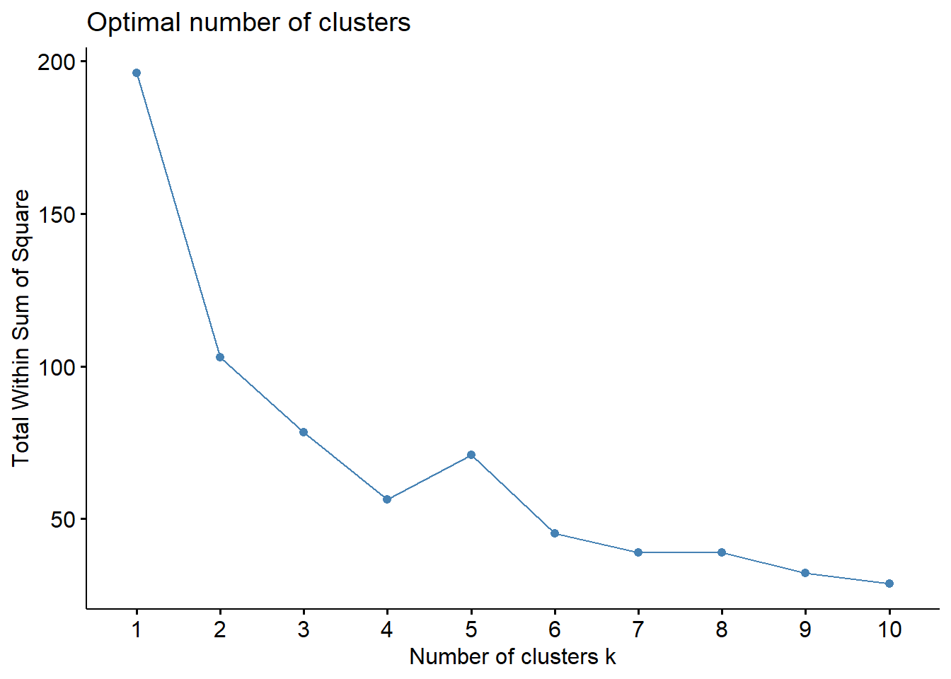
Here, you can see that the optimal number of clusters is 4, since this is the ‘elbow’ or bend in the plot, indicating that beyond this point, additional clusters will not futher reduce the total within sum of squares.

28.3 Compute clusters with k=4

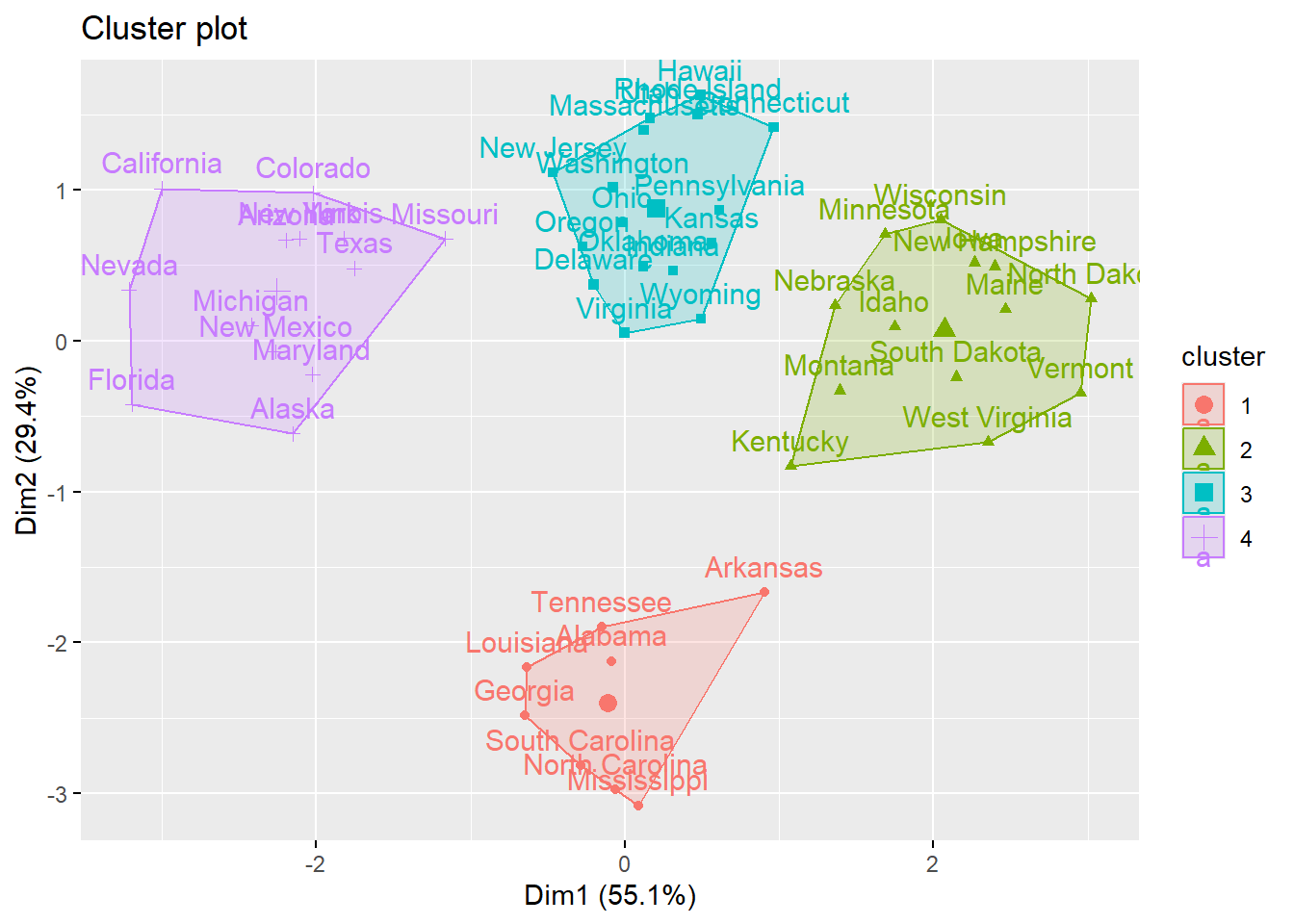
Here, you can see 4 clusters were computed of sizes 13, 13, 8, and 16.

# Set seed for reproducible results
set.seed(123)

# Run k-means algorithm
# Nstart = # random starting positions; I chose 20
km <- kmeans(df.scaled, 4, nstart = 20)

print(km)

K-means clustering with 4 clusters of sizes 8, 13, 16, 13

Cluster means:
      Murder    Assault   UrbanPop        Rape
1  1.4118898  0.8743346 -0.8145211  0.01927104
2 -0.9615407 -1.1066010 -0.9301069 -0.96676331
3 -0.4894375 -0.3826001  0.5758298 -0.26165379
4  0.6950701  1.0394414  0.7226370  1.27693964

Clustering vector:
       Alabama         Alaska        Arizona       Arkansas     California 
             1              4              4              1              4 
      Colorado    Connecticut       Delaware        Florida        Georgia 
             4              3              3              4              1 
        Hawaii          Idaho       Illinois        Indiana           Iowa 
             3              2              4              3              2 
        Kansas       Kentucky      Louisiana          Maine       Maryland 
             3              2              1              2              4 
 Massachusetts       Michigan      Minnesota    Mississippi       Missouri 
             3              4              2              1              4 
       Montana       Nebraska         Nevada  New Hampshire     New Jersey 
             2              2              4              2              3 
    New Mexico       New York North Carolina   North Dakota           Ohio 
             4              4              1              2              3 
      Oklahoma         Oregon   Pennsylvania   Rhode Island South Carolina 
             3              3              3              3              1 
  South Dakota      Tennessee          Texas           Utah        Vermont 
             2              1              4              3              2 
      Virginia     Washington  West Virginia      Wisconsin        Wyoming 
             3              3              2              2              3 

Within cluster sum of squares by cluster:
[1]  8.316061 11.952463 16.212213 19.922437
 (between_SS / total_SS =  71.2 %)

Available components:

[1] "cluster"      "centers"      "totss"        "withinss"     "tot.withinss"
[6] "betweenss"    "size"         "iter"         "ifault"      

28.4 Add the cluster number back to the dataset

df.cluster <- cbind(df, cluster=km$cluster)

head(df.cluster)

           Murder Assault UrbanPop Rape cluster
Alabama      13.2     236       58 21.2       1
Alaska       10.0     263       48 44.5       4
Arizona       8.1     294       80 31.0       4
Arkansas      8.8     190       50 19.5       1
California    9.0     276       91 40.6       4
Colorado      7.9     204       78 38.7       4

28.5 Plot results

Because there are 4 possible clusters (that is, more than 2 variables to plot on an XY axis), we can reduce the dimensions by applying PCA to the k-means result.

PCA will take the four clusters and output two new variables (that represent the original data) so it can plot the clusters on an XY axis. The function fviz_cluster in the factoextra package will do that for you.

Here, you can see how the states cluster together with respect to crime statistics.

fviz_cluster(km, data = df.cluster)