6  Naïve Bayes

# read in the data 
diab_pop <- readRDS(here::here('DATA/diab_pop.RDS'))

6.0.1 Reminders about the Data

tibble::tribble(
  ~"Variable in Data", ~"Definition", ~"Data Type",
  'seqn', 'Respondent sequence number', 'Identifier',
  'riagendr', 'Gender', 'Categorical',
  'ridageyr', 'Age in years at screening', 'Continuous / Numerical',
  'ridreth1', 'Race/Hispanic origin', 'Categorical',
  'dmdeduc2', 'Education level', 'Adults 20+  - Categorical',
  'dmdmartl', 'Marital status', 'Categorical',
  'indhhin2', 'Annual household income', 'Categorical',
  'bmxbmi', 'Body Mass Index (kg/m**2)', 'Continuous / Numerical',
  'diq010', 'Doctor diagnosed diabetes', 'Categorical',
  'lbxglu', 'Fasting Glucose (mg/dL)', 'Continuous / Numerical'
  ) |>
  knitr::kable()

Variable in Data	Definition	Data Type
seqn	Respondent sequence number	Identifier
riagendr	Gender	Categorical
ridageyr	Age in years at screening	Continuous / Numerical
ridreth1	Race/Hispanic origin	Categorical
dmdeduc2	Education level	Adults 20+ - Categorical
dmdmartl	Marital status	Categorical
indhhin2	Annual household income	Categorical
bmxbmi	Body Mass Index (kg/m**2)	Continuous / Numerical
diq010	Doctor diagnosed diabetes	Categorical
lbxglu	Fasting Glucose (mg/dL)	Continuous / Numerical

6.0.2 Install if not Function

install_if_not <- function( list.of.packages ) {
  new.packages <- list.of.packages[!(list.of.packages %in% installed.packages()[,"Package"])]
  if(length(new.packages)) { install.packages(new.packages) } else { print(paste0("the package '", list.of.packages , "' is already installed")) }
}

6.1 The e1071 package

install_if_not('e1071')

[1] "the package 'e1071' is already installed"

library('e1071')

6.2 Split Data

library('caret')

Loading required package: ggplot2

Loading required package: lattice

diab_pop.no_na <- na.omit(diab_pop)
trainIndex <- createDataPartition(diab_pop.no_na$diq010, 
                                  list = FALSE , 
                                  p = .8)

train <- diab_pop.no_na[trainIndex, ]
test <- diab_pop.no_na[-trainIndex, ]

6.3 Make Formula

features <- colnames(train)[!colnames(train) %in% c('diq010', 'seqn')]
features_plus <- paste0(features, collapse = " + ")
my_formula <- paste0("diq010 ~ ", features_plus)

my_formula

[1] "diq010 ~ riagendr + ridageyr + ridreth1 + dmdeduc2 + dmdmartl + indhhin2 + bmxbmi + lbxglu"

6.4 Train Model

model_nb <- naiveBayes( as.formula(my_formula) , data=train)

summary(model_nb)

          Length Class  Mode     
apriori   2      table  numeric  
tables    8      -none- list     
levels    2      -none- character
isnumeric 8      -none- logical  
call      4      -none- call     

6.5 Score

class <- predict(model_nb, test)
probs <- predict(model_nb, test, 'raw')

test.scored <- cbind(test, class, probs)

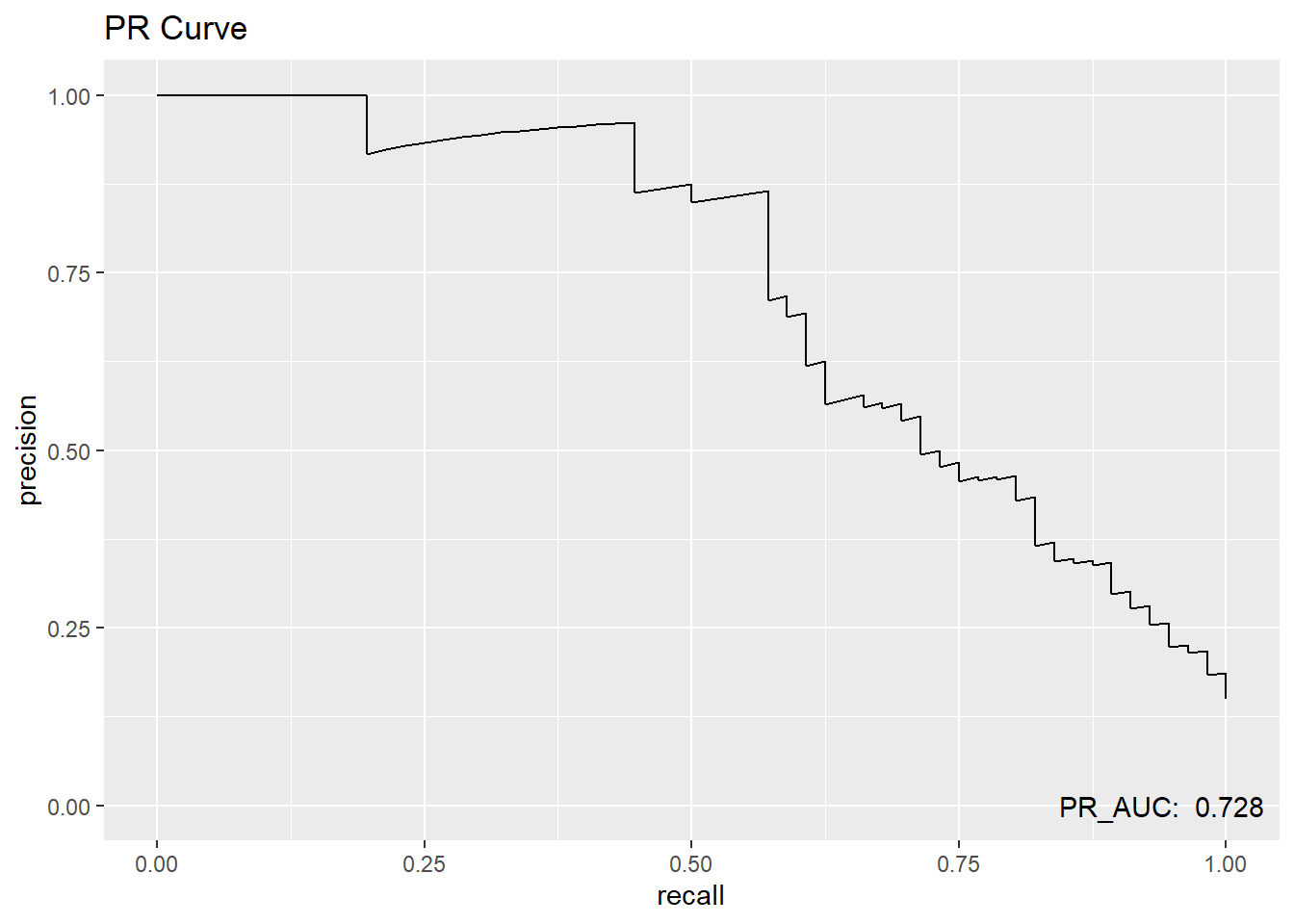
6.6 yardstick

library('dplyr')

Attaching package: 'dplyr'

The following objects are masked from 'package:stats':

    filter, lag

The following objects are masked from 'package:base':

    intersect, setdiff, setequal, union

library('yardstick')

Attaching package: 'yardstick'

The following objects are masked from 'package:caret':

    precision, recall, sensitivity, specificity

test.scored %>%
  conf_mat(truth=diq010, class)

             Truth
Prediction    Diabetes No Diabetes
  Diabetes          25           4
  No Diabetes       31         315

test.scored %>%
  conf_mat(truth=diq010, class) %>%
  autoplot()

test.scored %>%
  conf_mat(truth=diq010, class) %>%
  summary()

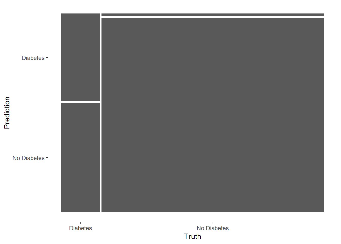
# A tibble: 13 × 3
   .metric              .estimator .estimate
   <chr>                <chr>          <dbl>
 1 accuracy             binary        0.907 
 2 kap                  binary        0.542 
 3 sens                 binary        0.446 
 4 spec                 binary        0.987 
 5 ppv                  binary        0.862 
 6 npv                  binary        0.910 
 7 mcc                  binary        0.579 
 8 j_index              binary        0.434 
 9 bal_accuracy         binary        0.717 
10 detection_prevalence binary        0.0773
11 precision            binary        0.862 
12 recall               binary        0.446 
13 f_meas               binary        0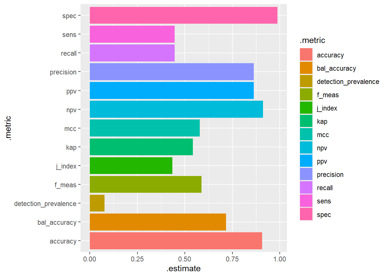.588 

test.scored %>%
  conf_mat(truth=diq010, class) %>%
  summary() %>%
  ggplot(aes(y=.metric, x=.estimate, fill=.metric)) +
  geom_bar(stat="identity")

test.scored %>%
  roc_curve(truth=diq010, Diabetes) %>%
  mutate(FPR = 1 - specificity) %>%
  mutate(TPR = sensitivity) %>%
  ggplot(aes(x=FPR, y=TPR)) +
  geom_line() +
  annotate("text", 
           x=.94, y=0, 
           label= paste("AUC: ",round(roc_auc(test.scored, truth=diq010, Diabetes)$.estimate,3))) +
  ggtitle("ROC Curve")

test.scored %>%
  pr_curve(truth=diq010, Diabetes) %>%
  ggplot(aes(x=recall, y=precision)) +
  geom_line() +
  annotate("text", 
           x=.94, y=0, 
           label= paste("PR_AUC: ",round(pr_auc(test.scored, truth=diq010, Diabetes)$.estimate,3))) +
  ggtitle("PR Curve")

test.scored %>%
  gain_curve(truth=diq010, Diabetes) %>%
  autoplot()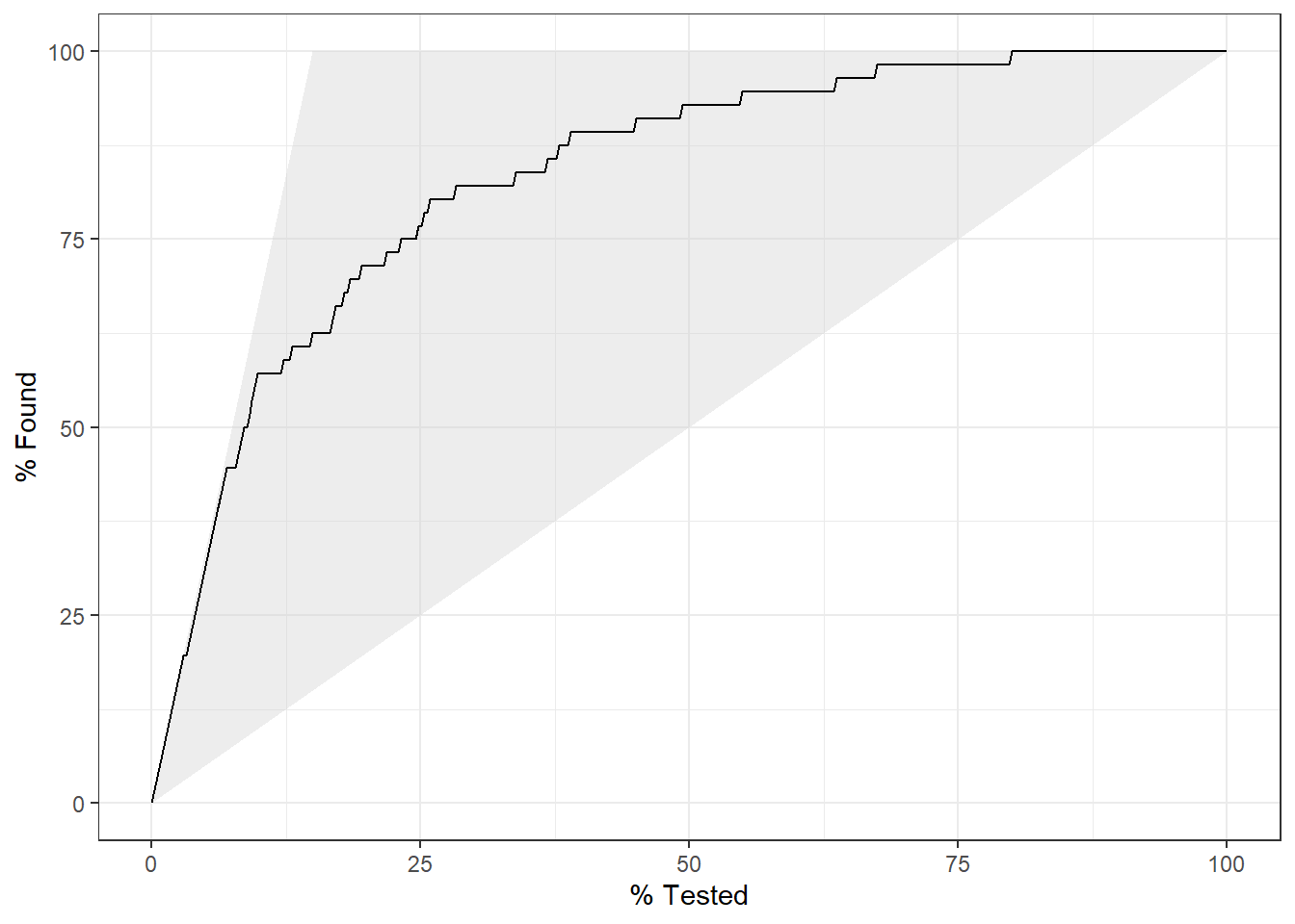

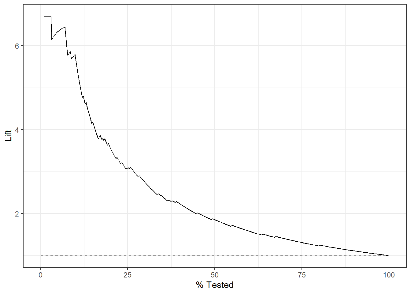
test.scored %>%
  lift_curve(truth=diq010, Diabetes) %>%
  autoplot()