Attaching package: 'yardstick'

The following objects are masked from 'package:caret':

    precision, recall, sensitivity, specificity

The following object is masked from 'package:readr':

    spec
# THIS IS NOT A GREAT IDEA options(warn=-1)# I have this on, there is an expected warning ## "prediction from a rank-deficient fit may be misleading"## without this option on the output is very difficult to read
                                                     statistic value
1                                       Number of by-variables     1
2                         Number of non-by variables in common     9
3                                 Number of variables compared     9
4                           Number of variables in x but not y     0
5                           Number of variables in y but not x     3
6        Number of variables compared with some values unequal     0
7           Number of variables compared with all values equal     9
8                             Number of observations in common     0
9                        Number of observations in x but not y   394
10                       Number of observations in y but not x   168
11 Number of observations with some compared variables unequal     0
12    Number of observations with all compared variables equal     0
13                                    Number of values unequal     0
      seqn         riagendr     ridageyr                   ridreth1
 Min.   :84166   Male  : 0   Min.   :21.00   MexicanAmerican   : 0
 1st Qu.:85920   Female:29   1st Qu.:32.00   Other Hispanic    : 0
 Median :89041               Median :48.00   Non-Hispanic White:29
 Mean   :88741               Mean   :50.14   Non-Hispanic Black: 0
 3rd Qu.:91064               3rd Qu.:61.00   Other             : 0
 Max.   :92970               Max.   :80.00

                       dmdeduc2                 dmdmartl
 Less than 9th grade       : 0   Married            :19
 Grades 9-11th             : 1   Widowed            : 3
 High school graduate/GED  : 4   Divorced           : 2
 Some college or AA degrees:14   Separated          : 0
 College grad or above     :10   Never married      : 1
                                 Living with partner: 4

              indhhin2      bmxbmi              diq010       lbxglu
 $75,000-$99,999  :29   Min.   :16.70   Diabetes   : 1   Min.   : 80.0
 $0-$4,999        : 0   1st Qu.:23.70   No Diabetes:28   1st Qu.: 92.0
 $5,000-$9,999    : 0   Median :26.80                    Median : 99.0
 $10,000-$14,999  : 0   Mean   :30.05                    Mean   :104.3
 $15,000-$19,999  : 0   3rd Qu.:33.30                    3rd Qu.:105.0
 less than $20,000: 0   Max.   :63.60                    Max.   :207.0
 (Other)          : 0
Compare Object

Function Call:
arsenal::comparedf(x = X3$Training_Data, y = X5$Training_Data)

Shared: 10 non-by variables and 21 observations.
Not shared: 0 variables and 626 observations.

Differences found in 10/10 variables compared.
0 variables compared have non-identical attributes.
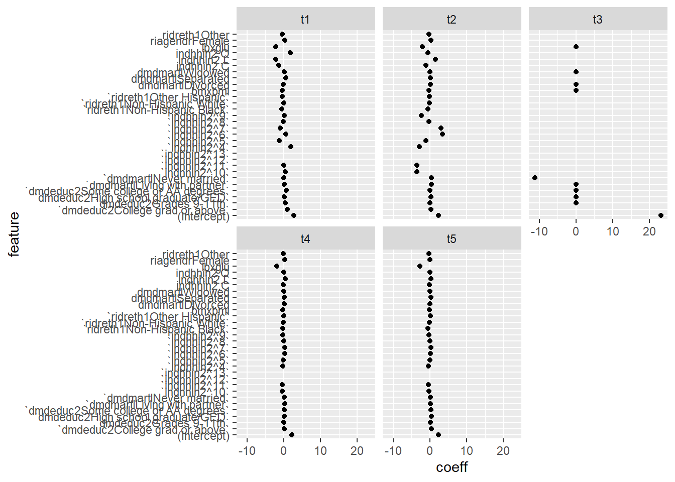
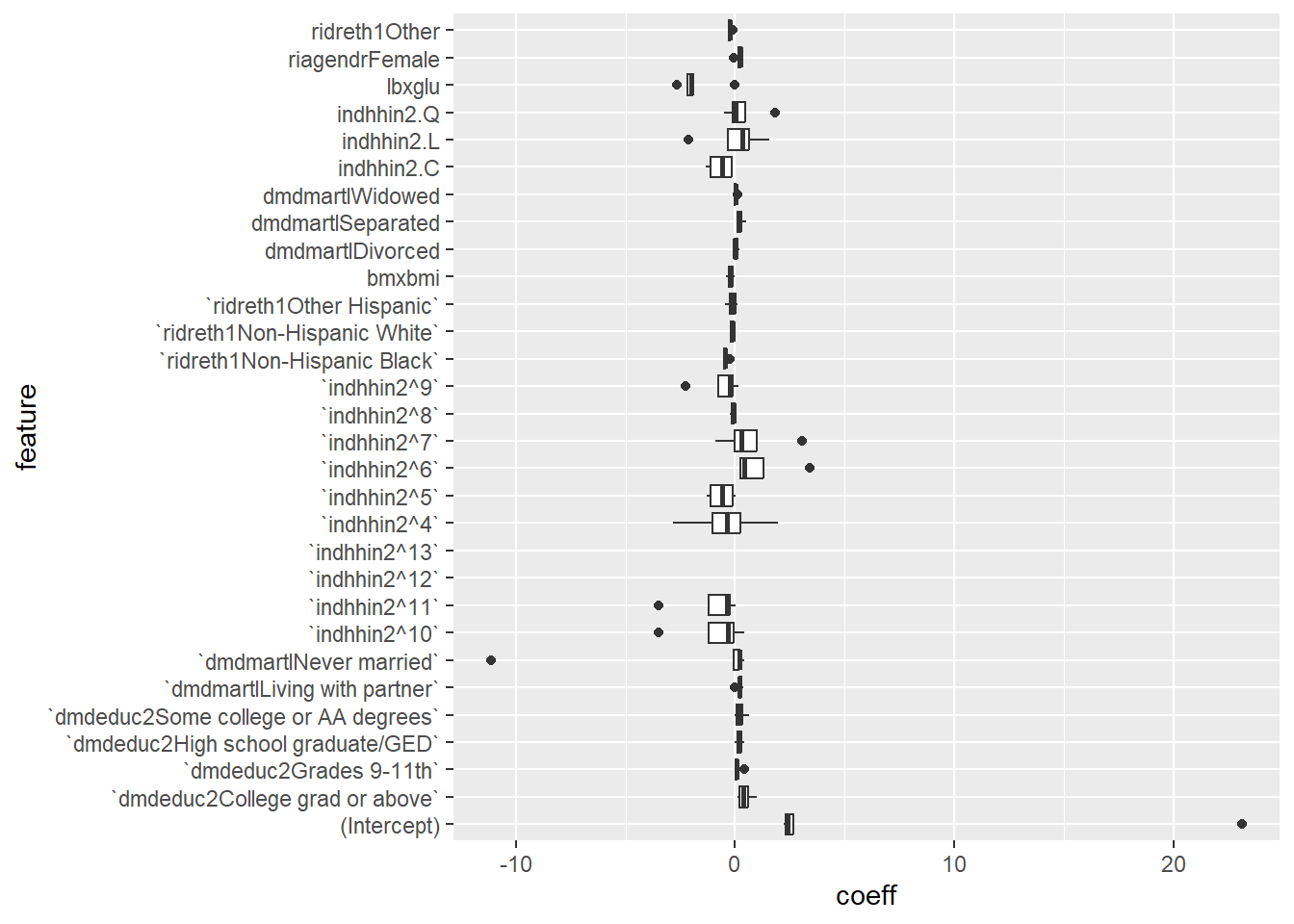
18.5 Compare Coefficents across all samples
X1$CoEff
# A tibble: 30 × 2
   feature                                coeff
   <chr>                                  <dbl>
 1 (Intercept)                           2.68
 2 riagendrFemale                        0.223
 3 `ridreth1Other Hispanic`             -0.451
 4 `ridreth1Non-Hispanic White`         -0.0250
 5 `ridreth1Non-Hispanic Black`         -0.483
 6 ridreth1Other                        -0.337
 7 `dmdeduc2Grades 9-11th`               0.420
 8 `dmdeduc2High school graduate/GED`    0.207
 9 `dmdeduc2Some college or AA degrees`  0.630
10 `dmdeduc2College grad or above`       0.980
# ℹ 20 more rows
Compare Object

Function Call:
arsenal::comparedf(x = t3, y = f3, by = c("seqn"))

Shared: 9 non-by variables and 0 observations.
Not shared: 0 variables and 1876 observations.

Differences found in 0/9 variables compared.
0 variables compared have non-identical attributes.
                                                     statistic value
1                                       Number of by-variables     1
2                         Number of non-by variables in common     9
3                                 Number of variables compared     9
4                           Number of variables in x but not y     0
5                           Number of variables in y but not x     0
6        Number of variables compared with some values unequal     0
7           Number of variables compared with all values equal     9
8                             Number of observations in common     0
9                        Number of observations in x but not y    29
10                       Number of observations in y but not x  1847
11 Number of observations with some compared variables unequal     0
12    Number of observations with all compared variables equal     0
13                                    Number of values unequal     0
Compare Object

Function Call:
arsenal::comparedf(x = X3$TEST.scored, y = f3, by = c("seqn"))

Shared: 9 non-by variables and 0 observations.
Not shared: 3 variables and 1855 observations.

Differences found in 0/9 variables compared.
0 variables compared have non-identical attributes.
                                                     statistic value
1                                       Number of by-variables     1
2                         Number of non-by variables in common     9
3                                 Number of variables compared     9
4                           Number of variables in x but not y     3
5                           Number of variables in y but not x     0
6        Number of variables compared with some values unequal     0
7           Number of variables compared with all values equal     9
8                             Number of observations in common     0
9                        Number of observations in x but not y     8
10                       Number of observations in y but not x  1847
11 Number of observations with some compared variables unequal     0
12    Number of observations with all compared variables equal     0
13                                    Number of values unequal     0
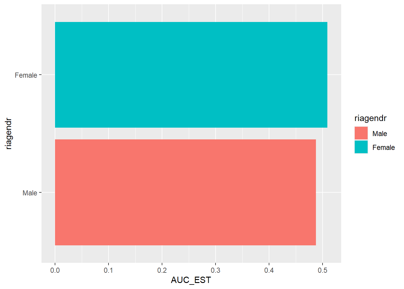
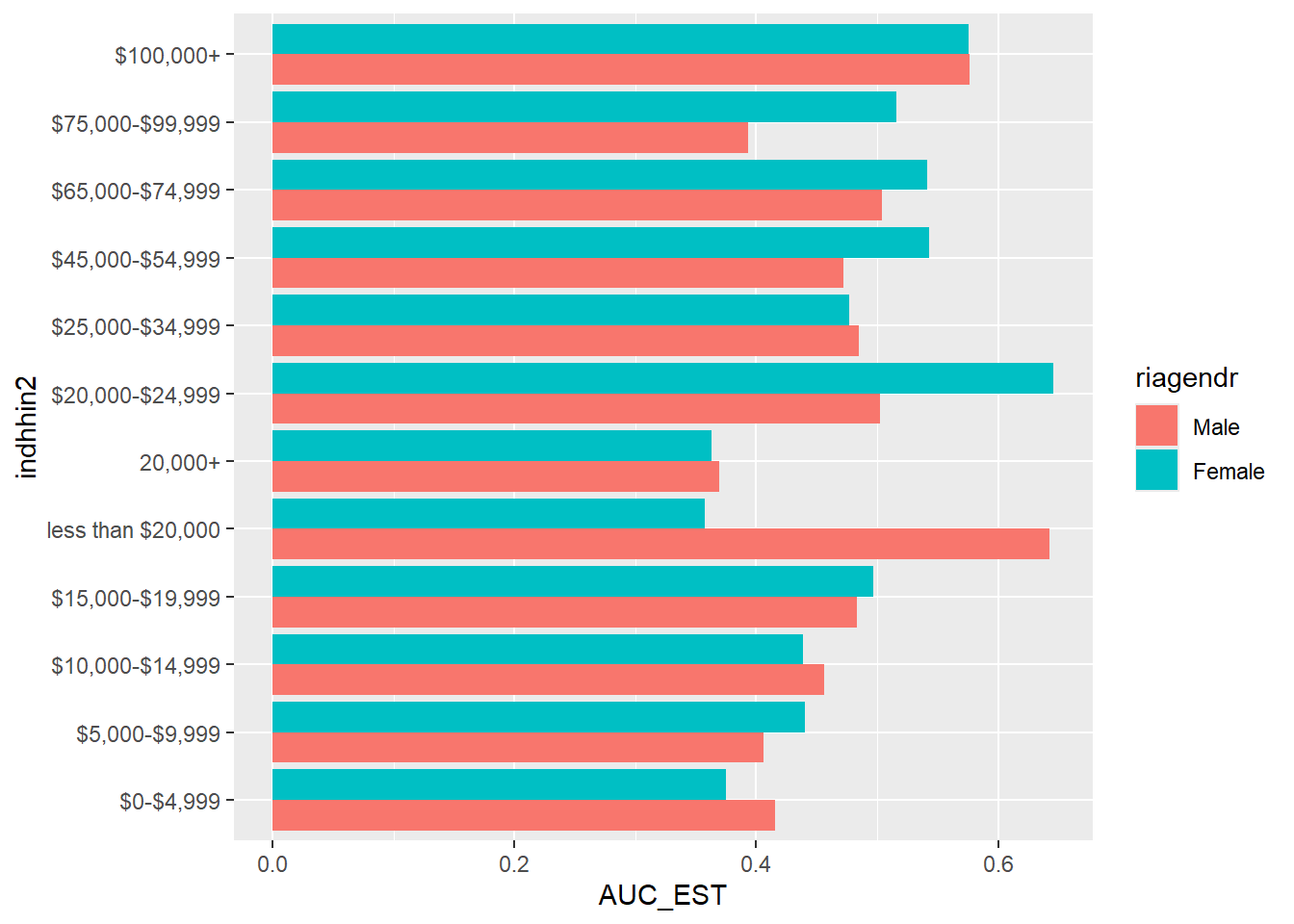
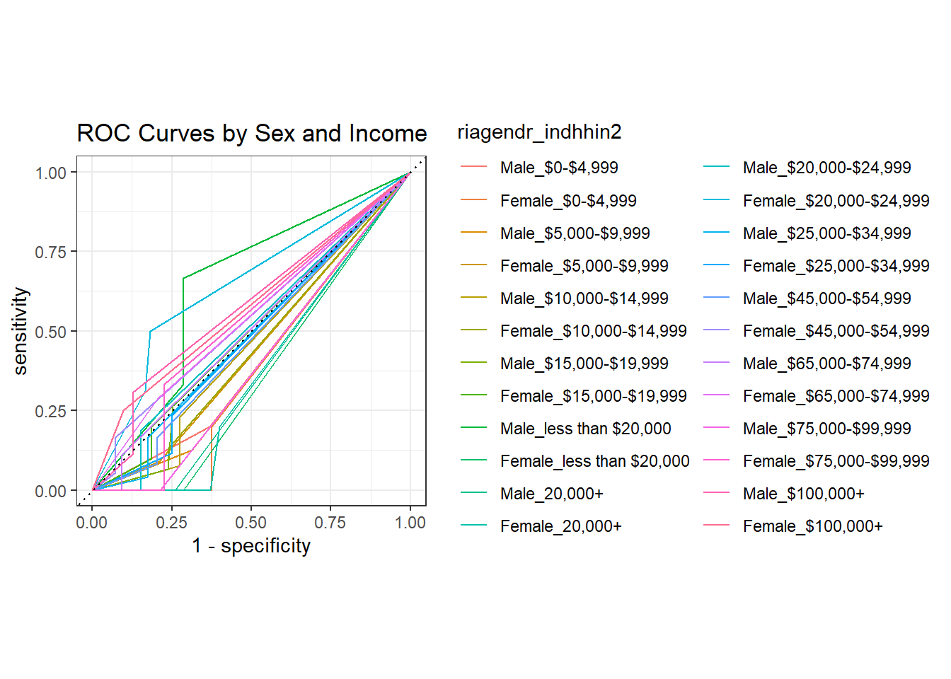
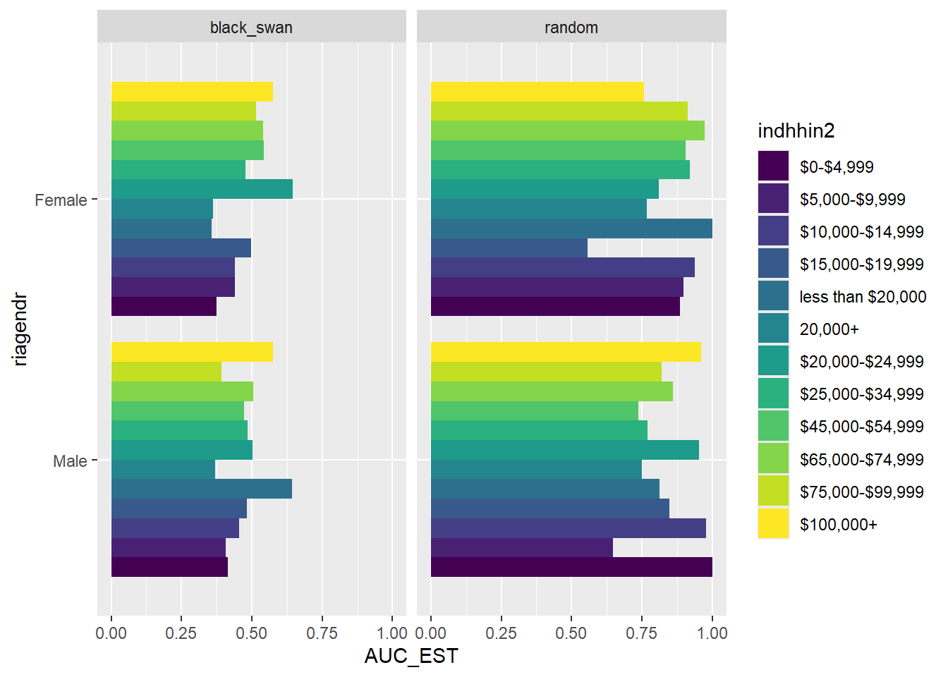
# A tibble: 24 × 3
   riagendr indhhin2          conf_mat
   <fct>    <ord>             <list>
 1 Male     $0-$4,999         <conf_mat>
 2 Male     $5,000-$9,999     <conf_mat>
 3 Male     $10,000-$14,999   <conf_mat>
 4 Male     $15,000-$19,999   <conf_mat>
 5 Male     less than $20,000 <conf_mat>
 6 Male     20,000+           <conf_mat>
 7 Male     $20,000-$24,999   <conf_mat>
 8 Male     $25,000-$34,999   <conf_mat>
 9 Male     $45,000-$54,999   <conf_mat>
10 Male     $65,000-$74,999   <conf_mat>
# ℹ 14 more rows
   riagendr               indhhin2
 Male  :12   $0-$4,999        : 2
 Female:12   $5,000-$9,999    : 2
             $10,000-$14,999  : 2
             $15,000-$19,999  : 2
             less than $20,000: 2
             20,000+          : 2
             (Other)          :12


 conf_mat.Length  conf_mat.Class  conf_mat.Mode
 1         conf_mat  list
 1         conf_mat  list
 1         conf_mat  list
 1         conf_mat  list
 1         conf_mat  list
 1         conf_mat  list
 1         conf_mat  list
 1         conf_mat  list
 1         conf_mat  list
 1         conf_mat  list
 1         conf_mat  list
 1         conf_mat  list
 1         conf_mat  list
 1         conf_mat  list
 1         conf_mat  list
 1         conf_mat  list
 1         conf_mat  list
 1         conf_mat  list
 1         conf_mat  list
 1         conf_mat  list
 1         conf_mat  list
 1         conf_mat  list
 1         conf_mat  list
 1         conf_mat  list
Compare Object

Function Call:
arsenal::comparedf(x = t2, y = f2, by = c("seqn"))

Shared: 9 non-by variables and 0 observations.
Not shared: 0 variables and 1876 observations.

Differences found in 0/9 variables compared.
0 variables compared have non-identical attributes.
                                                     statistic value
1                                       Number of by-variables     1
2                         Number of non-by variables in common     9
3                                 Number of variables compared     9
4                           Number of variables in x but not y     0
5                           Number of variables in y but not x     0
6        Number of variables compared with some values unequal     0
7           Number of variables compared with all values equal     9
8                             Number of observations in common     0
9                        Number of observations in x but not y   938
10                       Number of observations in y but not x   938
11 Number of observations with some compared variables unequal     0
12    Number of observations with all compared variables equal     0
13                                    Number of values unequal     0