9  k-Nearest Neighbors with caret

# read in the data 
diab_pop <- readRDS(here::here('DATA/diab_pop.RDS'))

9.0.1 Reminders about the Data

tibble::tribble(
  ~"Variable in Data", ~"Definition", ~"Data Type",
  'seqn', 'Respondent sequence number', 'Identifier',
  'riagendr', 'Gender', 'Categorical',
  'ridageyr', 'Age in years at screening', 'Continuous / Numerical',
  'ridreth1', 'Race/Hispanic origin', 'Categorical',
  'dmdeduc2', 'Education level', 'Adults 20+  - Categorical',
  'dmdmartl', 'Marital status', 'Categorical',
  'indhhin2', 'Annual household income', 'Categorical',
  'bmxbmi', 'Body Mass Index (kg/m**2)', 'Continuous / Numerical',
  'diq010', 'Doctor diagnosed diabetes', 'Categorical',
  'lbxglu', 'Fasting Glucose (mg/dL)', 'Continuous / Numerical'
  ) |>
  knitr::kable()

Variable in Data	Definition	Data Type
seqn	Respondent sequence number	Identifier
riagendr	Gender	Categorical
ridageyr	Age in years at screening	Continuous / Numerical
ridreth1	Race/Hispanic origin	Categorical
dmdeduc2	Education level	Adults 20+ - Categorical
dmdmartl	Marital status	Categorical
indhhin2	Annual household income	Categorical
bmxbmi	Body Mass Index (kg/m**2)	Continuous / Numerical
diq010	Doctor diagnosed diabetes	Categorical
lbxglu	Fasting Glucose (mg/dL)	Continuous / Numerical

9.0.2 Install if not Function

install_if_not <- function( list.of.packages ) {
  new.packages <- list.of.packages[!(list.of.packages %in% installed.packages()[,"Package"])]
  if(length(new.packages)) { install.packages(new.packages) } else { print(paste0("the package '", list.of.packages , "' is already installed")) }
}

9.1 Load tidyverse

library('tidyverse')

── Attaching core tidyverse packages ──────────────────────── tidyverse 2.0.0 ──
✔ dplyr     1.1.4     ✔ readr     2.1.5
✔ forcats   1.0.0     ✔ stringr   1.5.1
✔ ggplot2   3.5.1     ✔ tibble    3.2.1
✔ lubridate 1.9.3     ✔ tidyr     1.3.1
✔ purrr     1.0.2     
── Conflicts ────────────────────────────────────────── tidyverse_conflicts() ──
✖ dplyr::filter() masks stats::filter()
✖ dplyr::lag()    masks stats::lag()
ℹ Use the conflicted package (<http://conflicted.r-lib.org/>) to force all conflicts to become errors

levels(diab_pop$diq010) <- c("Diabetes", "No_Diabetes")

diab_pop.no_na_vals <- diab_pop %>% na.omit()

9.2 The caret package

library('caret')

Loading required package: lattice

Attaching package: 'caret'

The following object is masked from 'package:purrr':

    lift

# this will ensure our results are the same every run, 
# to randomize you may use: set.seed(Sys.time())

set.seed(8675309)

9.3 Split Data

# The createDataPartition function is used to create training and test sets

trainIndex <- createDataPartition(diab_pop.no_na_vals$diq010, 
                                  p = .6, 
                                  list = FALSE, 
                                  times = 1)

dm2.train <- diab_pop.no_na_vals[trainIndex, ]
dm2.test <- diab_pop.no_na_vals[-trainIndex, ]

9.4 Make Grid

# we will make a grid of values to test in cross-validation.
knnGrid <-  expand.grid(k = 1:15)

9.4.1 Optimize for Accuracy

9.4.1.1 The trainControl function

# the method here is cv for cross-validation you could try "repeatedcv"  for repeated cross-fold validation
fitControl <- trainControl(method = "cv", # uncomment for repeatedcv 
                           number = 10, 
                           # repeats = 10, # uncomment for repeatedcv 
                           ## Estimate class probabilities
                           classProbs = TRUE)

9.4.1.2 The train function

knnFit <- train(diq010 ~ ., # formula
                 data = dm2.train, # train data   
                 method = "knn", # method for caret see https://topepo.github.io/caret/available-models.html for list of models 
                 trControl = fitControl, 
                 tuneGrid = knnGrid,
                 metric = "Accuracy") ## Specify which metric to optimize

9.4.1.3 Results

knnFit

k-Nearest Neighbors 

1126 samples
   9 predictor
   2 classes: 'Diabetes', 'No_Diabetes' 

No pre-processing
Resampling: Cross-Validated (10 fold) 
Summary of sample sizes: 1013, 1013, 1013, 1014, 1013, 1013, ... 
Resampling results across tuning parameters:

  k   Accuracy   Kappa     
   1  0.8552070  0.38286631
   2  0.8471871  0.32674490
   3  0.8693979  0.32082482
   4  0.8649652  0.25745853
   5  0.8703303  0.24645605
   6  0.8614728  0.17410430
   7  0.8614570  0.12685254
   8  0.8641277  0.15354040
   9  0.8605563  0.11030512
  10  0.8570006  0.07271797
  11  0.8561157  0.06507766
  12  0.8543458  0.04587766
  13  0.8525759  0.02878628
  14  0.8507980  0.00960000
  15  0.8516909  0.01985641

Accuracy was used to select the optimal model using the largest value.
The final value used for the model was k = 5.

plot(knnFit)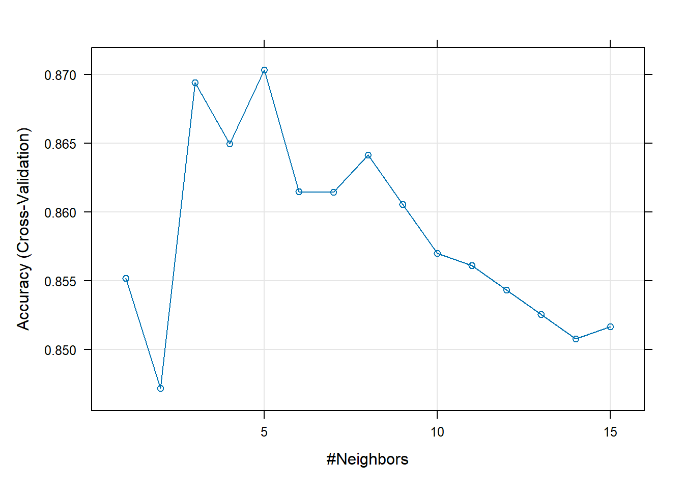

str(knnFit,1)

List of 25
 $ method      : chr "knn"
 $ modelInfo   :List of 13
 $ modelType   : chr "Classification"
 $ results     :'data.frame':   15 obs. of  5 variables:
 $ pred        : NULL
 $ bestTune    :'data.frame':   1 obs. of  1 variable:
 $ call        : language train.formula(form = diq010 ~ ., data = dm2.train, method = "knn", trControl = fitControl,      tuneGrid = knnGri| __truncated__
 $ dots        : list()
 $ metric      : chr "Accuracy"
 $ control     :List of 27
 $ finalModel  :List of 8
  ..- attr(*, "class")= chr "knn3"
 $ preProcess  : NULL
 $ trainingData:'data.frame':   1126 obs. of  10 variables:
 $ ptype       :'data.frame':   0 obs. of  9 variables:
 $ resample    :'data.frame':   10 obs. of  3 variables:
 $ resampledCM :'data.frame':   150 obs. of  6 variables:
 $ perfNames   : chr [1:2] "Accuracy" "Kappa"
 $ maximize    : logi TRUE
 $ yLimits     : NULL
 $ times       :List of 3
 $ levels      : chr [1:2] "Diabetes" "No_Diabetes"
  ..- attr(*, "ordered")= logi FALSE
 $ terms       :Classes 'terms', 'formula'  language diq010 ~ seqn + riagendr + ridageyr + ridreth1 + dmdeduc2 + dmdmartl +      indhhin2 + bmxbmi + lbxglu
  .. ..- attr(*, "variables")= language list(diq010, seqn, riagendr, ridageyr, ridreth1, dmdeduc2, dmdmartl, indhhin2,      bmxbmi, lbxglu)
  .. ..- attr(*, "factors")= int [1:10, 1:9] 0 1 0 0 0 0 0 0 0 0 ...
  .. .. ..- attr(*, "dimnames")=List of 2
  .. ..- attr(*, "term.labels")= chr [1:9] "seqn" "riagendr" "ridageyr" "ridreth1" ...
  .. ..- attr(*, "order")= int [1:9] 1 1 1 1 1 1 1 1 1
  .. ..- attr(*, "intercept")= int 1
  .. ..- attr(*, "response")= int 1
  .. ..- attr(*, ".Environment")=<environment: R_GlobalEnv> 
  .. ..- attr(*, "predvars")= language list(diq010, seqn, riagendr, ridageyr, ridreth1, dmdeduc2, dmdmartl, indhhin2,      bmxbmi, lbxglu)
  .. ..- attr(*, "dataClasses")= Named chr [1:10] "factor" "numeric" "factor" "numeric" ...
  .. .. ..- attr(*, "names")= chr [1:10] "diq010" "seqn" "riagendr" "ridageyr" ...
 $ coefnames   : chr [1:31] "seqn" "riagendrFemale" "ridageyr" "ridreth1Other Hispanic" ...
 $ contrasts   :List of 5
 $ xlevels     :List of 5
 - attr(*, "class")= chr [1:2] "train" "train.formula"

knnFit$finalModel  

5-nearest neighbor model
Training set outcome distribution:

   Diabetes No_Diabetes 
        169         957 

9.4.1.3.1 Score Test Data

# let's score the test set using this model
pred_class <- predict(knnFit, dm2.test,'raw')
probs <- predict(knnFit, dm2.test,'prob')

dm2.test.scored <- cbind(dm2.test, pred_class, probs)

glimpse(dm2.test.scored)

Rows: 750
Columns: 13
$ seqn        <dbl> 83734, 83737, 83757, 83761, 83789, 83820, 83822, 83823, 83…
$ riagendr    <fct> Male, Female, Female, Female, Male, Male, Female, Female, …
$ ridageyr    <dbl> 78, 72, 57, 24, 66, 70, 20, 29, 69, 71, 37, 49, 41, 54, 80…
$ ridreth1    <fct> Non-Hispanic White, MexicanAmerican, Other Hispanic, Other…
$ dmdeduc2    <fct> High school graduate/GED, Grades 9-11th, Less than 9th gra…
$ dmdmartl    <fct> Married, Separated, Separated, Never married, Living with …
$ indhhin2    <fct> "$20,000-$24,999", "$75,000-$99,999", "$20,000-$24,999", "…
$ bmxbmi      <dbl> 28.8, 28.6, 35.4, 25.3, 34.0, 27.0, 22.2, 29.7, 28.2, 27.6…
$ diq010      <fct> Diabetes, No_Diabetes, Diabetes, No_Diabetes, No_Diabetes,…
$ lbxglu      <dbl> 84, 107, 398, 95, 113, 94, 80, 102, 105, 76, 79, 126, 110,…
$ pred_class  <fct> No_Diabetes, No_Diabetes, No_Diabetes, No_Diabetes, No_Dia…
$ Diabetes    <dbl> 0.0, 0.0, 0.4, 0.0, 0.0, 0.0, 0.0, 0.0, 0.0, 0.2, 0.0, 0.2…
$ No_Diabetes <dbl> 1.0, 1.0, 0.6, 1.0, 1.0, 1.0, 1.0, 1.0, 1.0, 0.8, 1.0, 0.8…

9.4.1.3.2 Use yardstick for model metrics

# yardstick 
library('yardstick')

Attaching package: 'yardstick'

The following objects are masked from 'package:caret':

    precision, recall, sensitivity, specificity

The following object is masked from 'package:readr':

    spec

9.4.1.3.3 Confusion Matrix

dm2.test.scored %>% 
  conf_mat(truth=diq010 , pred_class)

             Truth
Prediction    Diabetes No_Diabetes
  Diabetes          14           3
  No_Diabetes       98         635

dm2.test.scored %>% 
  conf_mat(truth=diq010 , pred_class) %>%
  summary()

# A tibble: 13 × 3
   .metric              .estimator .estimate
   <chr>                <chr>          <dbl>
 1 accuracy             binary        0.865 
 2 kap                  binary        0.185 
 3 sens                 binary        0.125 
 4 spec                 binary        0.995 
 5 ppv                  binary        0.824 
 6 npv                  binary        0.866 
 7 mcc                  binary        0.288 
 8 j_index              binary        0.120 
 9 bal_accuracy         binary        0.560 
10 detection_prevalence binary        0.0227
11 precision            binary        0.824 
12 recall               binary        0.125 
13 f_meas               binary        0.217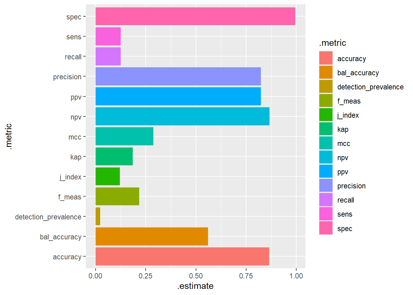 

dm2.test.scored %>% 
  conf_mat(truth=diq010 , pred_class) %>% 
  summary() %>%
  ggplot(aes(y=.metric, x=.estimate, fill=.metric)) +
  geom_bar(stat="identity")

9.4.1.3.4 ROC Curve

knnFit.roc_auc <- dm2.test.scored %>% 
  roc_auc(truth=diq010 , Diabetes)

knnFit.roc_auc

# A tibble: 1 × 3
  .metric .estimator .estimate
  <chr>   <chr>          <dbl>
1 roc_auc binary         0.728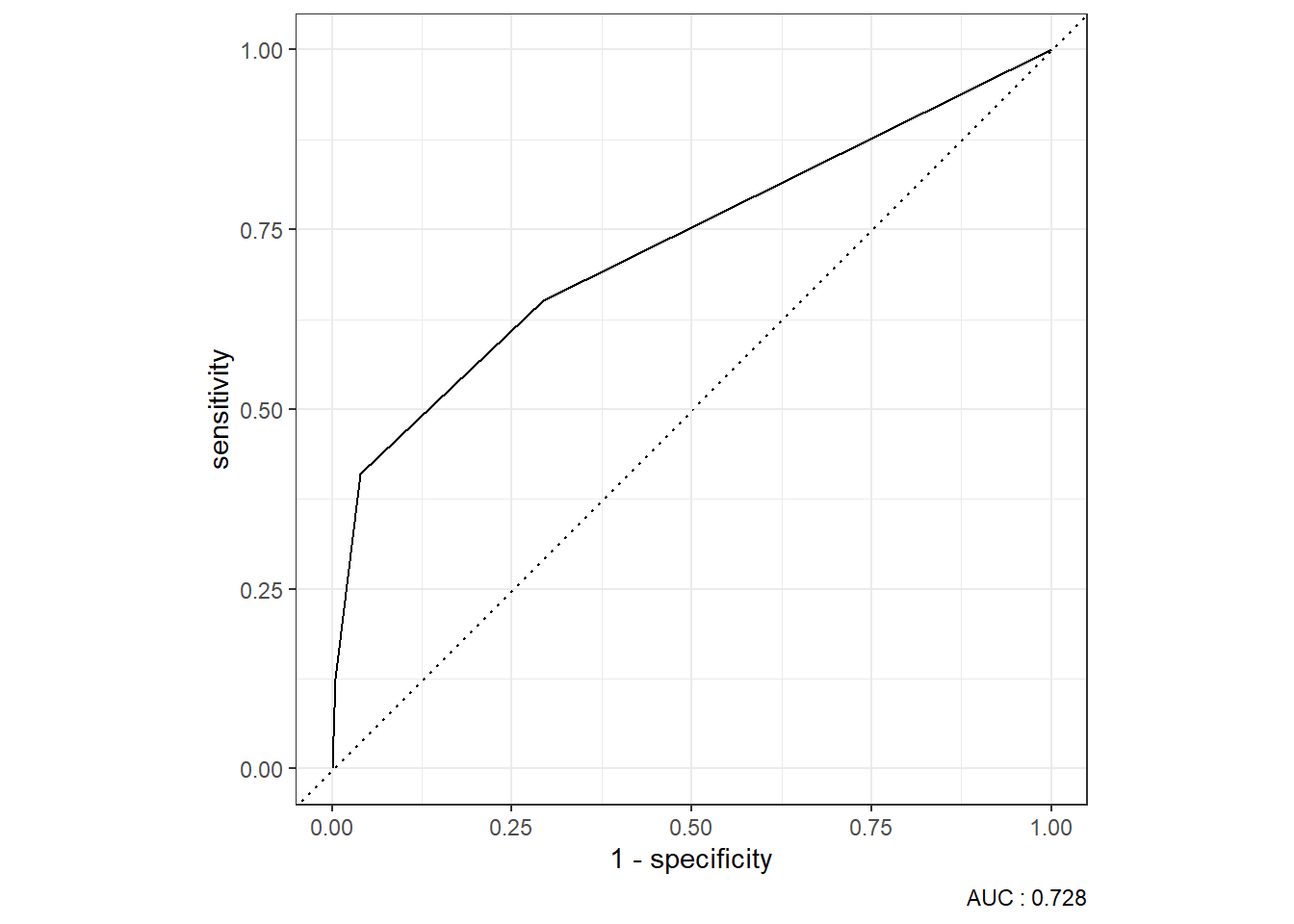

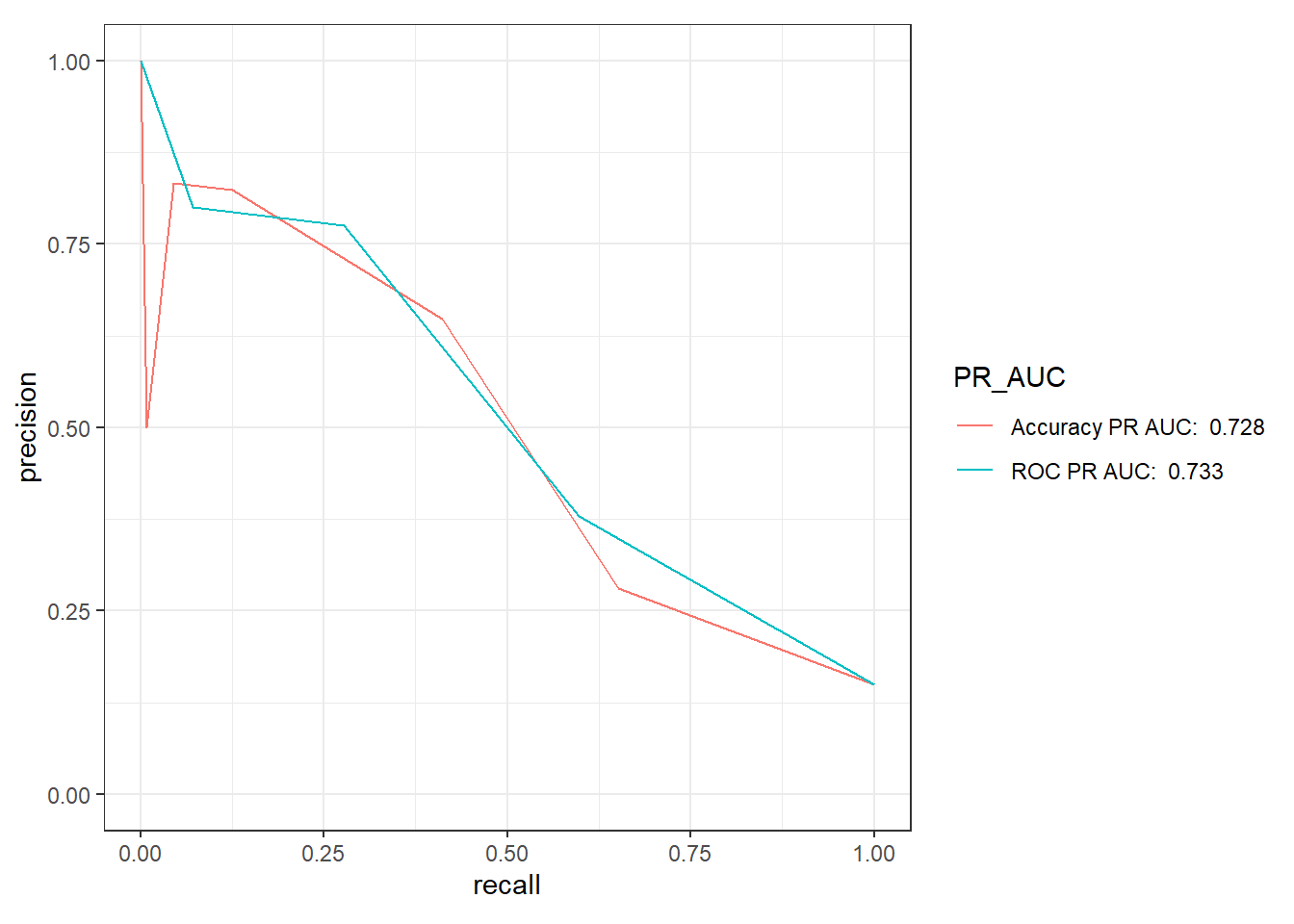
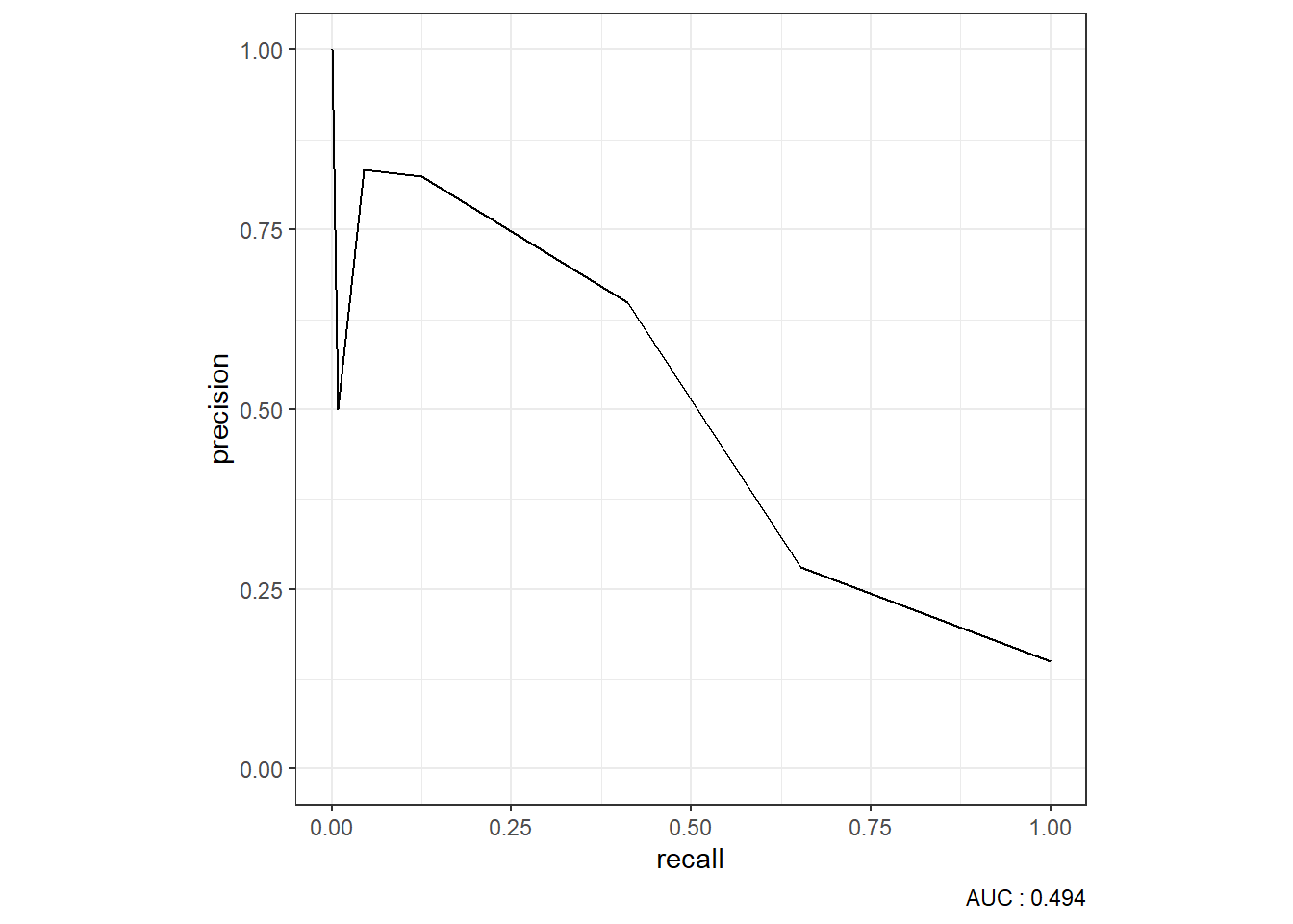
knnFit.roc_curve <- dm2.test.scored %>% 
  roc_curve(truth=diq010 , Diabetes) %>%
  autoplot() + 
  labs(caption = paste0("AUC : ", round(knnFit.roc_auc$.estimate,3)))

knnFit.roc_curve

9.4.1.3.5 Precision-Recall Curve

knnFit.pr_auc <- dm2.test.scored %>% 
  pr_auc(truth=diq010 , Diabetes) 

knnFit.pr_curve <- dm2.test.scored %>% 
  pr_curve(truth=diq010 , Diabetes) %>%
  autoplot() +
  labs(caption = paste0("AUC : ",  round(knnFit.pr_auc$.estimate,3)))

knnFit.pr_curve

9.4.2 Optimize for ROC

9.4.2.1 The trainControl function

# the method here is cv for cross-validation you could try "repeatedcv"  for repeated cross-fold validation
fitControl <- trainControl(method = "cv", # uncomment for repeatedcv 
                           number = 10, 
                           # repeats = 10, # uncomment for repeatedcv 
                           ## Estimate class probabilities
                           classProbs = TRUE,
                           summaryFunction=twoClassSummary)

9.4.2.2 The train function

knnFit_ROC <- train(diq010 ~ ., # formula
                 data = dm2.train, # train data   
                 method = "knn", # method for caret see https://topepo.github.io/caret/available-models.html for list of models 
                 trControl = fitControl, 
                 tuneGrid = knnGrid,
                 metric = "ROC") ## Specify which metric to optimize

9.4.2.3 Results

knnFit_ROC

k-Nearest Neighbors 

1126 samples
   9 predictor
   2 classes: 'Diabetes', 'No_Diabetes' 

No pre-processing
Resampling: Cross-Validated (10 fold) 
Summary of sample sizes: 1013, 1014, 1014, 1014, 1013, 1013, ... 
Resampling results across tuning parameters:

  k   ROC        Sens         Spec     
   1  0.6683833  0.395220588  0.9415461
   2  0.7051856  0.389705882  0.9404276
   3  0.7176461  0.265441176  0.9749342
   4  0.7156281  0.224632353  0.9812061
   5  0.7006004  0.153308824  0.9937281
   6  0.6966088  0.135294118  0.9937390
   7  0.6899122  0.076470588  0.9979167
   8  0.6780983  0.076470588  0.9968750
   9  0.6762613  0.058823529  1.0000000
  10  0.6752873  0.052941176  0.9989583
  11  0.6677884  0.035294118  1.0000000
  12  0.6583659  0.023529412  1.0000000
  13  0.6547260  0.011764706  1.0000000
  14  0.6528311  0.005882353  1.0000000
  15  0.6497179  0.011764706  1.0000000

ROC was used to select the optimal model using the largest value.
The final value used for the model was k = 3.

plot(knnFit_ROC)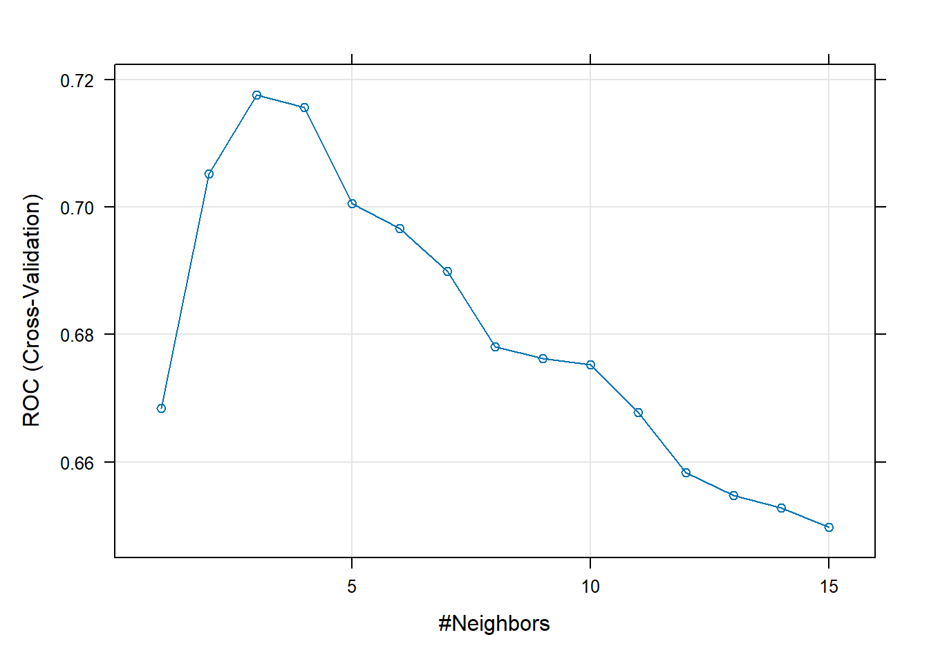

str(knnFit_ROC,1)

List of 25
 $ method      : chr "knn"
 $ modelInfo   :List of 13
 $ modelType   : chr "Classification"
 $ results     :'data.frame':   15 obs. of  7 variables:
 $ pred        : NULL
 $ bestTune    :'data.frame':   1 obs. of  1 variable:
 $ call        : language train.formula(form = diq010 ~ ., data = dm2.train, method = "knn", trControl = fitControl,      tuneGrid = knnGri| __truncated__
 $ dots        : list()
 $ metric      : chr "ROC"
 $ control     :List of 27
 $ finalModel  :List of 8
  ..- attr(*, "class")= chr "knn3"
 $ preProcess  : NULL
 $ trainingData:'data.frame':   1126 obs. of  10 variables:
 $ ptype       :'data.frame':   0 obs. of  9 variables:
 $ resample    :'data.frame':   10 obs. of  4 variables:
 $ resampledCM :'data.frame':   150 obs. of  6 variables:
 $ perfNames   : chr [1:3] "ROC" "Sens" "Spec"
 $ maximize    : logi TRUE
 $ yLimits     : NULL
 $ times       :List of 3
 $ levels      : chr [1:2] "Diabetes" "No_Diabetes"
  ..- attr(*, "ordered")= logi FALSE
 $ terms       :Classes 'terms', 'formula'  language diq010 ~ seqn + riagendr + ridageyr + ridreth1 + dmdeduc2 + dmdmartl +      indhhin2 + bmxbmi + lbxglu
  .. ..- attr(*, "variables")= language list(diq010, seqn, riagendr, ridageyr, ridreth1, dmdeduc2, dmdmartl, indhhin2,      bmxbmi, lbxglu)
  .. ..- attr(*, "factors")= int [1:10, 1:9] 0 1 0 0 0 0 0 0 0 0 ...
  .. .. ..- attr(*, "dimnames")=List of 2
  .. ..- attr(*, "term.labels")= chr [1:9] "seqn" "riagendr" "ridageyr" "ridreth1" ...
  .. ..- attr(*, "order")= int [1:9] 1 1 1 1 1 1 1 1 1
  .. ..- attr(*, "intercept")= int 1
  .. ..- attr(*, "response")= int 1
  .. ..- attr(*, ".Environment")=<environment: R_GlobalEnv> 
  .. ..- attr(*, "predvars")= language list(diq010, seqn, riagendr, ridageyr, ridreth1, dmdeduc2, dmdmartl, indhhin2,      bmxbmi, lbxglu)
  .. ..- attr(*, "dataClasses")= Named chr [1:10] "factor" "numeric" "factor" "numeric" ...
  .. .. ..- attr(*, "names")= chr [1:10] "diq010" "seqn" "riagendr" "ridageyr" ...
 $ coefnames   : chr [1:31] "seqn" "riagendrFemale" "ridageyr" "ridreth1Other Hispanic" ...
 $ contrasts   :List of 5
 $ xlevels     :List of 5
 - attr(*, "class")= chr [1:2] "train" "train.formula"

knnFit_ROC$finalModel  

3-nearest neighbor model
Training set outcome distribution:

   Diabetes No_Diabetes 
        169         957 

9.4.2.3.1 Score Test Data

# let's score the test set using this model
pred_class <- predict(knnFit_ROC, dm2.test, 'raw')
probs <- predict(knnFit_ROC, dm2.test, 'prob')

dm2.test.scored_ROC <- cbind(dm2.test, pred_class, probs)

glimpse(dm2.test.scored_ROC)

Rows: 750
Columns: 13
$ seqn        <dbl> 83734, 83737, 83757, 83761, 83789, 83820, 83822, 83823, 83…
$ riagendr    <fct> Male, Female, Female, Female, Male, Male, Female, Female, …
$ ridageyr    <dbl> 78, 72, 57, 24, 66, 70, 20, 29, 69, 71, 37, 49, 41, 54, 80…
$ ridreth1    <fct> Non-Hispanic White, MexicanAmerican, Other Hispanic, Other…
$ dmdeduc2    <fct> High school graduate/GED, Grades 9-11th, Less than 9th gra…
$ dmdmartl    <fct> Married, Separated, Separated, Never married, Living with …
$ indhhin2    <fct> "$20,000-$24,999", "$75,000-$99,999", "$20,000-$24,999", "…
$ bmxbmi      <dbl> 28.8, 28.6, 35.4, 25.3, 34.0, 27.0, 22.2, 29.7, 28.2, 27.6…
$ diq010      <fct> Diabetes, No_Diabetes, Diabetes, No_Diabetes, No_Diabetes,…
$ lbxglu      <dbl> 84, 107, 398, 95, 113, 94, 80, 102, 105, 76, 79, 126, 110,…
$ pred_class  <fct> No_Diabetes, No_Diabetes, Diabetes, No_Diabetes, No_Diabet…
$ Diabetes    <dbl> 0.0000000, 0.0000000, 0.6666667, 0.0000000, 0.0000000, 0.0…
$ No_Diabetes <dbl> 1.0000000, 1.0000000, 0.3333333, 1.0000000, 1.0000000, 1.0…

9.4.2.3.2 Use yardstick for model metrics

library('yardstick')

9.4.2.3.3 Confusion Matrix

dm2.test.scored_ROC %>% 
  conf_mat(truth=diq010 , pred_class)

             Truth
Prediction    Diabetes No_Diabetes
  Diabetes          31           9
  No_Diabetes       81         629

dm2.test.scored_ROC %>% 
  conf_mat(truth=diq010 , pred_class) %>%
  summary()

# A tibble: 13 × 3
   .metric              .estimator .estimate
   <chr>                <chr>          <dbl>
 1 accuracy             binary        0.88  
 2 kap                  binary        0.357 
 3 sens                 binary        0.277 
 4 spec                 binary        0.986 
 5 ppv                  binary        0.775 
 6 npv                  binary        0.886 
 7 mcc                  binary        0.417 
 8 j_index              binary        0.263 
 9 bal_accuracy         binary        0.631 
10 detection_prevalence binary        0.0533
11 precision            binary        0.775 
12 recall               binary        0.277 
13 f_meas               binary        0.408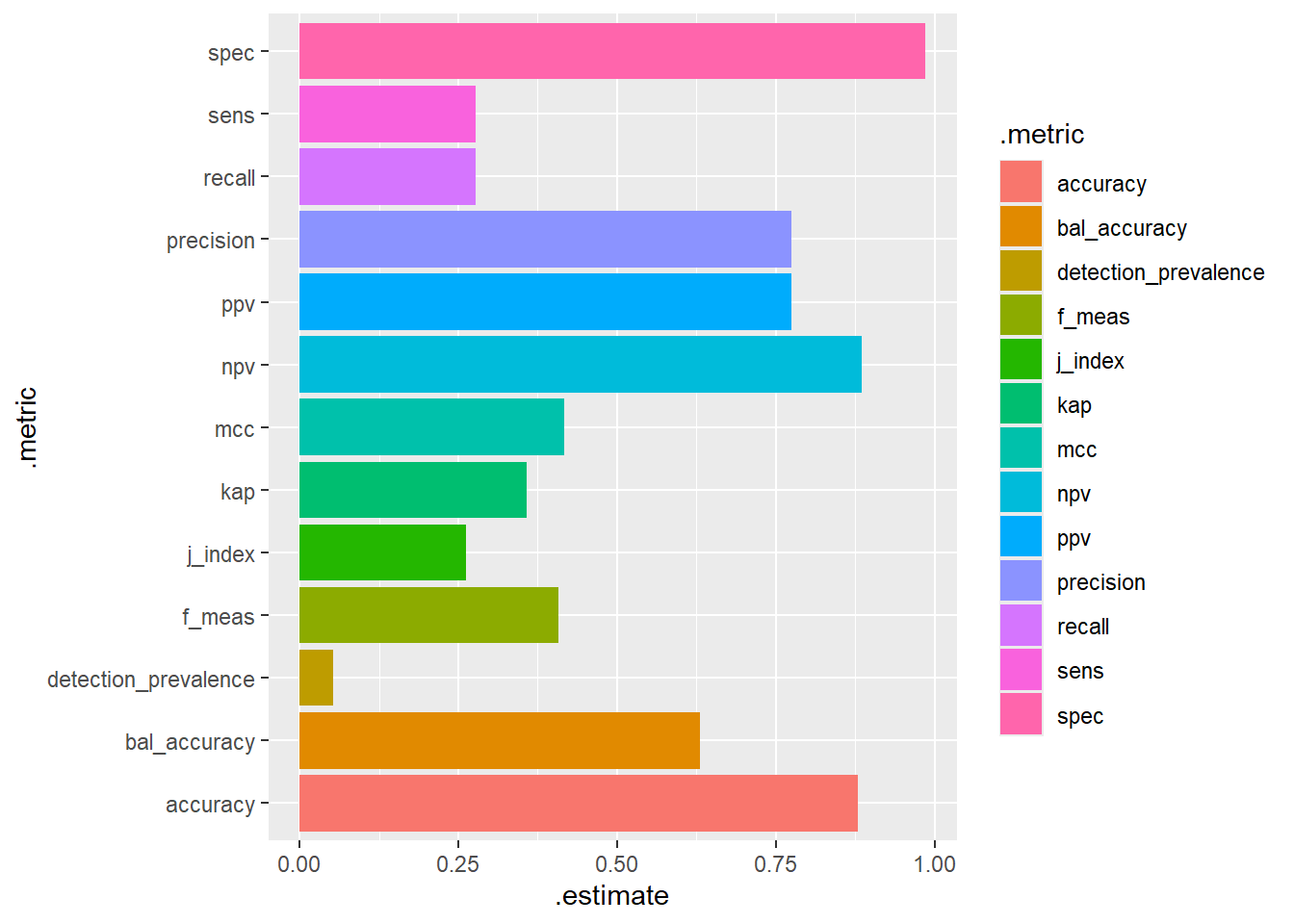 

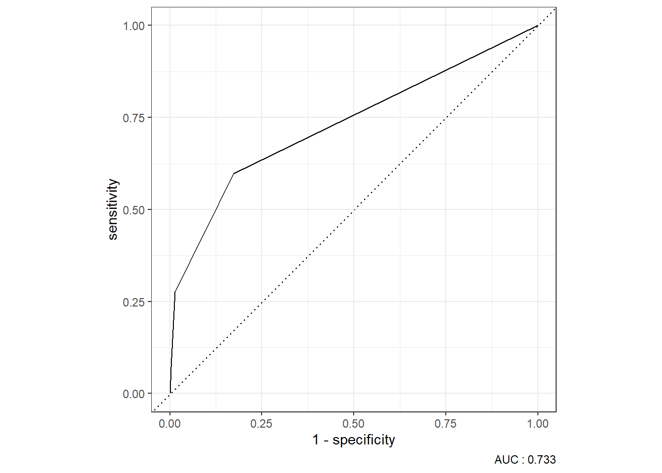
dm2.test.scored_ROC %>% 
  conf_mat(truth=diq010 , pred_class) %>% 
  summary() %>%
  ggplot(aes(y=.metric, x=.estimate, fill=.metric)) +
  geom_bar(stat="identity")

9.4.2.3.4 ROC Curve

knnFit_ROC.roc_auc <- dm2.test.scored_ROC %>% 
  roc_auc(truth=diq010 , Diabetes)

dm2.test.scored_ROC %>% 
  roc_curve(truth=diq010 , Diabetes) %>%
  autoplot() + 
  labs(caption = paste0("AUC : ", round(knnFit_ROC.roc_auc$.estimate,3)))

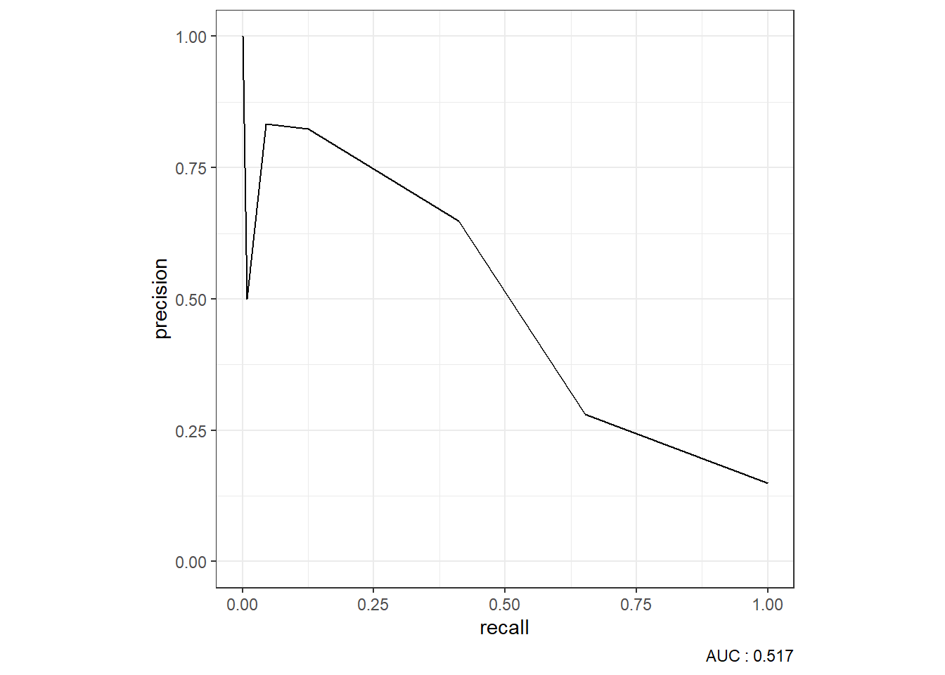
9.4.2.3.5 Precision-Recall Curve

knnFit_ROC.pr_auc <- dm2.test.scored_ROC %>% 
  pr_auc(truth=diq010 , Diabetes) 

dm2.test.scored %>% 
  pr_curve(truth=diq010 , Diabetes) %>%
  autoplot() +
  labs(caption = paste0("AUC : ",  round(knnFit_ROC.pr_auc$.estimate,3)))

9.5 Compare Results

knn_Fit_compare <- rbind(
  dm2.test.scored %>% mutate(model = "Accuracy"),
  dm2.test.scored_ROC %>% mutate(model = "ROC")
  )

9.5.1 Confusion Matrix

knn_Fit_compare %>% 
  group_by(model) %>%
  conf_mat(truth=diq010 , pred_class) %>%
  ungroup() %>%
  pull(conf_mat) %>%
  map(summary) %>%
  bind_rows(.id = "model") %>%
  mutate(model = if_else(model == 1, "Accuracy", "ROC")) %>%
  ggplot(aes(y=.metric, x=.estimate, fill=model, color = .metric)) +
  geom_bar(stat="identity", position = 'dodge')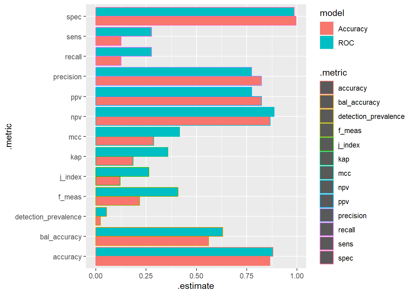

9.5.2 ROC Curve

knn_Fit_compare_AUC <- knn_Fit_compare %>% 
  group_by(model) %>%
  roc_auc(truth=diq010 , Diabetes) %>%
  mutate(AUC = paste(model, " AUC: ", round(.estimate,3))) %>%
  ungroup()

knn_Fit_compare %>% 
  left_join(knn_Fit_compare_AUC) %>%
  group_by(AUC) %>%
  roc_curve(truth=diq010 , Diabetes) %>%
  autoplot()

Joining with `by = join_by(model)`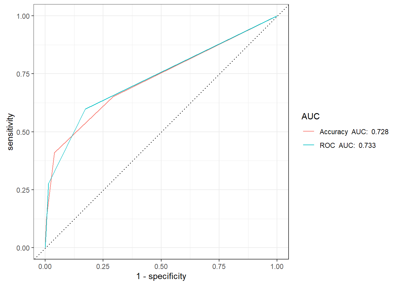

9.5.3 Precision-Recall Curve

knn_Fit_compare_PR <- knn_Fit_compare %>% 
  group_by(model) %>%
  roc_auc(truth=diq010 , Diabetes) %>%
  mutate(PR_AUC = paste(model, "PR AUC: ", round(.estimate,3))) %>%
  ungroup() 

knn_Fit_compare %>% 
  left_join(knn_Fit_compare_PR) %>%
  group_by(PR_AUC) %>%
  pr_curve(truth=diq010 , Diabetes) %>%
  autoplot()

Joining with `by = join_by(model)`

9.5.4 Lift

knn_Fit_compare %>% 
  group_by(model) %>%
  lift_curve(truth=diq010 , Diabetes) %>%
  autoplot()

9.5.5 Gain

knn_Fit_compare %>% 
  group_by(model) %>%
  gain_curve(truth=diq010 , Diabetes) %>%
  autoplot()