21 Read in the Data

#Decision Trees

\(~\)

diab_pop <- readRDS('C:/Users/jkyle/Documents/GitHub/Intro_Jeff_Data_Science/DATA/diab_pop.RDS')

\(~\)

21.1 Reminders

###The Data

#### Variable in Data - Definition - Data Type
##### seqn - Respondent sequence number - Identifier
##### riagendr - Gender - Categorical
##### ridageyr - Age in years at screening - Continuous / Numerical
##### ridreth1 - Race/Hispanic origin  - Categorical
##### dmdeduc2 - Education level - Adults 20+  - Categorical
##### dmdmartl - Marital status  - Categorical
##### indhhin2 - Annual household income  - Categorical
##### bmxbmi - Body Mass Index (kg/m**2) - Continuous / Numerical
##### diq010 - Doctor diagnosed diabetes - Categorical / Target
##### lbxglu - Fasting Glucose (mg/dL) - Continuous / Numerical

\(~\)

21.1.1 Install if not Function

install_if_not <- function( list.of.packages ) {
  new.packages <- list.of.packages[!(list.of.packages %in% installed.packages()[,"Package"])]
  if(length(new.packages)) { install.packages(new.packages) } else { print(paste0("the package '", list.of.packages , "' is already installed")) }
}

\(~\)

21.2 Data Prep

One thing we notice is there are a large number of missing values, take for lbxglu or example. For this example we will omit any values that have an ‘NA’ value, but we could also employ a missing value imputation strategy:

21.2.1 EDA and Imputation

library('tidyverse')

── Attaching core tidyverse packages ──────────────────────── tidyverse 2.0.0 ──
✔ dplyr     1.1.4     ✔ readr     2.1.5
✔ forcats   1.0.0     ✔ stringr   1.5.1
✔ ggplot2   3.5.1     ✔ tibble    3.2.1
✔ lubridate 1.9.3     ✔ tidyr     1.3.1
✔ purrr     1.0.2     
── Conflicts ────────────────────────────────────────── tidyverse_conflicts() ──
✖ dplyr::filter() masks stats::filter()
✖ dplyr::lag()    masks stats::lag()
ℹ Use the conflicted package (<http://conflicted.r-lib.org/>) to force all conflicts to become errors

diab_pop %>% 
  mutate( lbxglu_miss = ifelse(is.na(lbxglu),"missing","reported_value") ) %>%
  group_by(lbxglu_miss) %>%
  summarise( cnt= n() )

# A tibble: 2 × 2
  lbxglu_miss      cnt
  <chr>          <int>
1 missing         3267
2 reported_value  2452

# We could impute these values with 0 and add a flag indicating so:

diab_pop_impute0glu <- diab_pop %>% 
  mutate( lbxglu_miss = ifelse(is.na(lbxglu),"imputed_with_0","reported_value") ) %>%
  mutate( lbxglu = ifelse(is.na(lbxglu),0,lbxglu) )

glimpse(diab_pop_impute0glu)

Rows: 5,719
Columns: 11
$ seqn        <dbl> 83732, 83733, 83734, 83735, 83736, 83737, 83741, 83742, 83…
$ riagendr    <fct> Male, Male, Male, Female, Female, Female, Male, Female, Ma…
$ ridageyr    <dbl> 62, 53, 78, 56, 42, 72, 22, 32, 56, 46, 45, 30, 67, 67, 57…
$ ridreth1    <fct> Non-Hispanic White, Non-Hispanic White, Non-Hispanic White…
$ dmdeduc2    <fct> College grad or above, High school graduate/GED, High scho…
$ dmdmartl    <fct> Married, Divorced, Married, Living with partner, Divorced,…
$ indhhin2    <fct> "$65,000-$74,999", "$15,000-$19,999", "$20,000-$24,999", "…
$ bmxbmi      <dbl> 27.8, 30.8, 28.8, 42.4, 20.3, 28.6, 28.0, 28.2, 33.6, 27.6…
$ diq010      <fct> Diabetes, No Diabetes, Diabetes, No Diabetes, No Diabetes,…
$ lbxglu      <dbl> 0, 101, 84, 0, 84, 107, 95, 0, 0, 0, 84, 0, 130, 284, 398,…
$ lbxglu_miss <chr> "imputed_with_0", "reported_value", "reported_value", "imp…

# For this example we will omit any rows with any missing values:

diab_pop.no_na_vals <- diab_pop %>% na.omit()

glimpse(diab_pop.no_na_vals)

Rows: 1,876
Columns: 10
$ seqn     <dbl> 83733, 83734, 83737, 83750, 83754, 83755, 83757, 83761, 83787…
$ riagendr <fct> Male, Male, Female, Male, Female, Male, Female, Female, Femal…
$ ridageyr <dbl> 53, 78, 72, 45, 67, 67, 57, 24, 68, 66, 56, 37, 20, 24, 80, 7…
$ ridreth1 <fct> Non-Hispanic White, Non-Hispanic White, MexicanAmerican, Othe…
$ dmdeduc2 <fct> High school graduate/GED, High school graduate/GED, Grades 9-…
$ dmdmartl <fct> Divorced, Married, Separated, Never married, Married, Widowed…
$ indhhin2 <fct> "$15,000-$19,999", "$20,000-$24,999", "$75,000-$99,999", "$65…
$ bmxbmi   <dbl> 30.8, 28.8, 28.6, 24.1, 43.7, 28.8, 35.4, 25.3, 33.5, 34.0, 2…
$ diq010   <fct> No Diabetes, Diabetes, No Diabetes, No Diabetes, No Diabetes,…
$ lbxglu   <dbl> 101, 84, 107, 84, 130, 284, 398, 95, 111, 113, 397, 100, 94, …

\(~\)

21.3 Split Data with `caret`

We will want to split our data into two main sets: a training set to train the model and a testing set used to estimate model performance metrics.

install_if_not('caret')

[1] "the package 'caret' is already installed"

library('caret')

Loading required package: lattice


Attaching package: 'caret'

The following object is masked from 'package:purrr':

    lift

# this will ensure our results are the same every run, to randomize you may use: `set.seed(Sys.time())` or `set.seed(runif(1))`
set.seed(8675309)


# The createDataPartition function is used to create training and test sets

trainIndex <- createDataPartition(diab_pop.no_na_vals$diq010, 
                                  p = .6, 
                                  list = FALSE, 
                                  times = 1)

\(~\)

21.3.1 Define the Training Set

diab_pop.no_na_vals.train <- diab_pop.no_na_vals[trainIndex, ]

# Notice the size of the overall dataset
dim(diab_pop.no_na_vals)

[1] 1876   10

# and the size of our training set:
.6*nrow(diab_pop.no_na_vals)

[1] 1125.6

nrow(diab_pop.no_na_vals.train)

[1] 1126

\(~\)

21.3.2 Define the Testing Set

diab_pop.no_na_vals.test <- diab_pop.no_na_vals[-trainIndex, ]

nrow(diab_pop.no_na_vals) - .6*nrow(diab_pop.no_na_vals)

[1] 750.4

dim(diab_pop.no_na_vals.test)

[1] 750  10

\(~\)

21.4 Fit Decision Trees with `rpart`

train_set <- diab_pop.no_na_vals.train

install_if_not('rpart')

[1] "the package 'rpart' is already installed"

library('rpart')

### diq010 ~ riagendr + ridageyr + ridreth1 + dmdeduc2 + dmdmartl + indhhin2 + bmxbmi + lbxglu 
### diq010 ~ ridreth1 + lbxglu

tree_1 <- rpart(diq010 ~ riagendr + ridageyr + ridreth1 + dmdeduc2 + dmdmartl + indhhin2 + bmxbmi + lbxglu, 
                data = train_set,
                method="class",
                #parms = list(split = 'information'),
                control = rpart.control(minsplit = 1, 
                                        minbucket = 1, #round(minsplit/3)
                                        cp = 0.006, #3*10^(-3), 
                                        maxcompete = 4, 
                                        maxsurrogate = 5, 
                                        usesurrogate = 2, 
                                        xval = 10,
                                        surrogatestyle = 0, 
                                        maxdepth = 30))

tree_1

n= 1126 

node), split, n, loss, yval, (yprob)
      * denotes terminal node

  1) root 1126 169 No Diabetes (0.15008881 0.84991119)  
    2) lbxglu>=135 132  31 Diabetes (0.76515152 0.23484848)  
      4) lbxglu>=154.5 96  13 Diabetes (0.86458333 0.13541667)  
        8) indhhin2=$0-$4,999,$5,000-$9,999,$10,000-$14,999,$20,000-$24,999,$25,000-$34,999,$45,000-$54,999,$65,000-$74,999,$75,000-$99,999,$100,000+ 78   7 Diabetes (0.91025641 0.08974359) *
        9) indhhin2=$15,000-$19,999,20,000+,less than $20,000 18   6 Diabetes (0.66666667 0.33333333)  
         18) ridageyr>=49 15   3 Diabetes (0.80000000 0.20000000)  
           36) bmxbmi< 39.4 13   1 Diabetes (0.92307692 0.07692308) *
           37) bmxbmi>=39.4 2   0 No Diabetes (0.00000000 1.00000000) *
         19) ridageyr< 49 3   0 No Diabetes (0.00000000 1.00000000) *
      5) lbxglu< 154.5 36  18 Diabetes (0.50000000 0.50000000)  
       10) indhhin2=$25,000-$34,999,$65,000-$74,999,20,000+,$100,000+ 13   2 Diabetes (0.84615385 0.15384615) *
       11) indhhin2=$5,000-$9,999,$10,000-$14,999,$15,000-$19,999,$20,000-$24,999,$45,000-$54,999,less than $20,000,$75,000-$99,999 23   7 No Diabetes (0.30434783 0.69565217)  
         22) dmdmartl=Married,Divorced 14   7 Diabetes (0.50000000 0.50000000)  
           44) ridageyr>=63.5 8   2 Diabetes (0.75000000 0.25000000) *
           45) ridageyr< 63.5 6   1 No Diabetes (0.16666667 0.83333333) *
         23) dmdmartl=Widowed,Never married,Living with partner 9   0 No Diabetes (0.00000000 1.00000000) *
    3) lbxglu< 135 994  68 No Diabetes (0.06841046 0.93158954)  
      6) lbxglu>=113.5 146  34 No Diabetes (0.23287671 0.76712329)  
       12) indhhin2=$0-$4,999,$5,000-$9,999,$20,000-$24,999,less than $20,000 35  17 No Diabetes (0.48571429 0.51428571)  
         24) bmxbmi>=30.55 20   7 Diabetes (0.65000000 0.35000000)  
           48) lbxglu< 132 18   5 Diabetes (0.72222222 0.27777778) *
           49) lbxglu>=132 2   0 No Diabetes (0.00000000 1.00000000) *
         25) bmxbmi< 30.55 15   4 No Diabetes (0.26666667 0.73333333)  
           50) dmdmartl=Married,Separated 6   2 Diabetes (0.66666667 0.33333333)  
            100) bmxbmi< 26.8 4   0 Diabetes (1.00000000 0.00000000) *
            101) bmxbmi>=26.8 2   0 No Diabetes (0.00000000 1.00000000) *
           51) dmdmartl=Widowed,Divorced,Never married,Living with partner 9   0 No Diabetes (0.00000000 1.00000000) *
       13) indhhin2=$10,000-$14,999,$15,000-$19,999,$25,000-$34,999,$45,000-$54,999,$65,000-$74,999,20,000+,$75,000-$99,999,$100,000+ 111  17 No Diabetes (0.15315315 0.84684685)  
         26) ridageyr>=73.5 18   7 No Diabetes (0.38888889 0.61111111)  
           52) lbxglu>=124 6   1 Diabetes (0.83333333 0.16666667) *
           53) lbxglu< 124 12   2 No Diabetes (0.16666667 0.83333333) *
         27) ridageyr< 73.5 93  10 No Diabetes (0.10752688 0.89247312) *
      7) lbxglu< 113.5 848  34 No Diabetes (0.04009434 0.95990566)  
       14) lbxglu< 78.5 19   6 No Diabetes (0.31578947 0.68421053)  
         28) indhhin2=$0-$4,999,$5,000-$9,999 3   0 Diabetes (1.00000000 0.00000000) *
         29) indhhin2=$15,000-$19,999,$20,000-$24,999,$25,000-$34,999,$45,000-$54,999,$65,000-$74,999,20,000+,less than $20,000,$75,000-$99,999,$100,000+ 16   3 No Diabetes (0.18750000 0.81250000)  
           58) ridageyr>=56 6   3 Diabetes (0.50000000 0.50000000)  
            116) ridageyr< 62.5 3   0 Diabetes (1.00000000 0.00000000) *
            117) ridageyr>=62.5 3   0 No Diabetes (0.00000000 1.00000000) *
           59) ridageyr< 56 10   0 No Diabetes (0.00000000 1.00000000) *
       15) lbxglu>=78.5 829  28 No Diabetes (0.03377563 0.96622437) *

plot(tree_1)

\(~\)

21.5 Better View with `rpart.plot`

install_if_not('rpart.plot')

[1] "the package 'rpart.plot' is already installed"

library('rpart.plot')
rpart.plot(tree_1)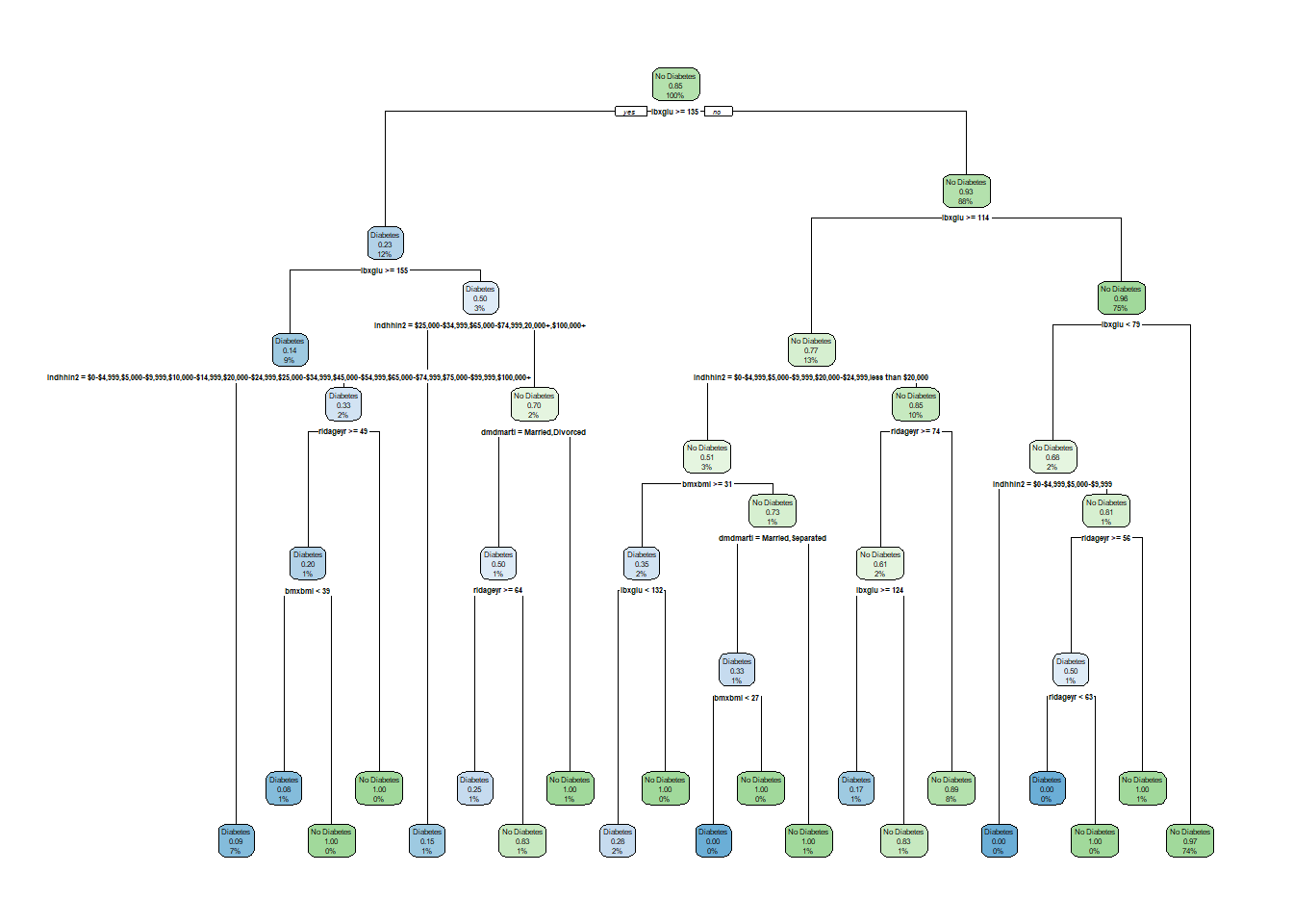

\(~\)

21.6 `rpart` output

str(tree_1,1)

List of 15
 $ frame              :'data.frame':    41 obs. of  9 variables:
 $ where              : Named int [1:1126] 41 41 32 4 41 7 41 41 41 31 ...
  ..- attr(*, "names")= chr [1:1126] "2" "11" "13" "14" ...
 $ call               : language rpart(formula = diq010 ~ riagendr + ridageyr + ridreth1 + dmdeduc2 + dmdmartl +      indhhin2 + bmxbmi + lbxglu, | __truncated__ ...
 $ terms              :Classes 'terms', 'formula'  language diq010 ~ riagendr + ridageyr + ridreth1 + dmdeduc2 + dmdmartl + indhhin2 +      bmxbmi + lbxglu
  .. ..- attr(*, "variables")= language list(diq010, riagendr, ridageyr, ridreth1, dmdeduc2, dmdmartl, indhhin2,      bmxbmi, lbxglu)
  .. ..- attr(*, "factors")= int [1:9, 1:8] 0 1 0 0 0 0 0 0 0 0 ...
  .. .. ..- attr(*, "dimnames")=List of 2
  .. ..- attr(*, "term.labels")= chr [1:8] "riagendr" "ridageyr" "ridreth1" "dmdeduc2" ...
  .. ..- attr(*, "order")= int [1:8] 1 1 1 1 1 1 1 1
  .. ..- attr(*, "intercept")= int 1
  .. ..- attr(*, "response")= int 1
  .. ..- attr(*, ".Environment")=<environment: R_GlobalEnv> 
  .. ..- attr(*, "predvars")= language list(diq010, riagendr, ridageyr, ridreth1, dmdeduc2, dmdmartl, indhhin2,      bmxbmi, lbxglu)
  .. ..- attr(*, "dataClasses")= Named chr [1:9] "factor" "factor" "numeric" "factor" ...
  .. .. ..- attr(*, "names")= chr [1:9] "diq010" "riagendr" "ridageyr" "ridreth1" ...
 $ cptable            : num [1:5, 1:5] 0.4142 0.02663 0.01183 0.00888 0.006 ...
  ..- attr(*, "dimnames")=List of 2
 $ method             : chr "class"
 $ parms              :List of 3
 $ control            :List of 9
 $ functions          :List of 3
 $ numresp            : int 4
 $ splits             : num [1:144, 1:5] 1126 1126 1126 1126 1126 ...
  ..- attr(*, "dimnames")=List of 2
 $ csplit             : int [1:78, 1:14] 1 1 1 1 1 1 3 3 1 3 ...
 $ variable.importance: Named num [1:8] 142.17 19.7 14.66 14.46 8.14 ...
  ..- attr(*, "names")= chr [1:8] "lbxglu" "indhhin2" "ridageyr" "bmxbmi" ...
 $ y                  : int [1:1126] 2 2 2 1 2 2 2 2 2 2 ...
 $ ordered            : Named logi [1:8] FALSE FALSE FALSE FALSE FALSE FALSE ...
  ..- attr(*, "names")= chr [1:8] "riagendr" "ridageyr" "ridreth1" "dmdeduc2" ...
 - attr(*, "xlevels")=List of 5
 - attr(*, "ylevels")= chr [1:2] "Diabetes" "No Diabetes"
 - attr(*, "class")= chr "rpart"

tree_1$splits

         count ncat     improve  index        adj
lbxglu    1126    1 113.1344112 135.00 0.00000000
ridageyr  1126    1  22.8255083  48.50 0.00000000
bmxbmi    1126    1   7.6602898  27.65 0.00000000
dmdeduc2  1126    5   5.7790434   1.00 0.00000000
dmdmartl  1126    6   5.7449142   2.00 0.00000000
lbxglu     132    1   6.9602273 154.50 0.00000000
bmxbmi     132    1   4.1704107  25.25 0.00000000
indhhin2   132   14   2.8812328   3.00 0.00000000
ridageyr   132    1   2.3778555  27.50 0.00000000
dmdmartl   132    6   1.8782314   4.00 0.00000000
ridageyr     0    1   0.7424242  27.50 0.05555556
bmxbmi       0    1   0.7424242  20.85 0.05555556
indhhin2     0   14   0.7348485   5.00 0.02777778
indhhin2    96   14   1.7355769   6.00 0.00000000
bmxbmi      96   -1   1.0405963  37.20 0.00000000
ridreth1    96    5   0.5720238   7.00 0.00000000
dmdmartl    96    6   0.5628608   8.00 0.00000000
ridageyr    96    1   0.5208333  61.50 0.00000000
bmxbmi       0    1   0.8333333  21.35 0.11111111
lbxglu       0   -1   0.8333333 393.50 0.11111111
ridageyr    18    1   3.2000000  49.00 0.00000000
bmxbmi      18   -1   3.2000000  39.40 0.00000000
dmdmartl    18    6   2.0000000   9.00 0.00000000
lbxglu      18    1   0.8000000 419.50 0.00000000
ridreth1    18    5   0.5000000  10.00 0.00000000
bmxbmi      15   -1   2.9538462  39.40 0.00000000
ridageyr    15    1   1.3714286  62.00 0.00000000
dmdmartl    15    6   1.3714286  11.00 0.00000000
dmdeduc2    15    5   0.6000000  12.00 0.00000000
ridreth1    15    5   0.4363636  13.00 0.00000000
indhhin2    36   14   4.8762542  14.00 0.00000000
dmdmartl    36    6   4.4307692  15.00 0.00000000
ridageyr    36    1   2.8928571  48.00 0.00000000
bmxbmi      36    1   2.8928571  25.35 0.00000000
dmdeduc2    36    5   1.0451613  16.00 0.00000000
dmdeduc2     0    5   0.6944444  17.00 0.15384615
bmxbmi       0    1   0.6944444  40.40 0.15384615
lbxglu       0    1   0.6666667 146.50 0.07692308
dmdmartl    23    6   2.7391304  18.00 0.00000000
ridageyr    23    1   1.9209486  63.50 0.00000000
ridreth1    23    5   1.8641304  19.00 0.00000000
dmdeduc2    23    5   0.8970252  20.00 0.00000000
bmxbmi      23   -1   0.8970252  37.60 0.00000000
ridreth1     0    5   0.7391304  21.00 0.33333333
ridageyr     0    1   0.6956522  32.00 0.22222222
dmdeduc2     0    5   0.6956522  22.00 0.22222222
indhhin2     0   14   0.6956522  23.00 0.22222222
bmxbmi       0   -1   0.6956522  31.05 0.22222222
ridageyr    14    1   2.3333333  63.50 0.00000000
lbxglu      14   -1   1.4000000 142.50 0.00000000
ridreth1    14    5   1.1666667  24.00 0.00000000
dmdmartl    14    6   1.1666667  25.00 0.00000000
bmxbmi      14   -1   1.1666667  37.80 0.00000000
ridreth1     0    5   0.7142857  26.00 0.33333333
dmdeduc2     0    5   0.7142857  27.00 0.33333333
indhhin2     0   14   0.7142857  28.00 0.33333333
bmxbmi       0   -1   0.7142857  37.80 0.33333333
riagendr     0    2   0.6428571  29.00 0.16666667
lbxglu     994    1   9.2582086 113.50 0.00000000
ridageyr   994    1   4.8704224  48.50 0.00000000
indhhin2   994   14   3.7854728  30.00 0.00000000
dmdeduc2   994    5   2.3395179  31.00 0.00000000
bmxbmi     994    1   2.1377841  48.55 0.00000000
indhhin2   146   14   5.8858765  32.00 0.00000000
ridageyr   146    1   2.3689223  73.50 0.00000000
dmdeduc2   146    5   1.9580029  33.00 0.00000000
lbxglu     146    1   1.5740855 121.50 0.00000000
ridreth1   146    5   1.5468950  34.00 0.00000000
bmxbmi       0   -1   0.7739726  22.25 0.05714286
bmxbmi      35    1   2.5190476  30.55 0.00000000
ridreth1    35    5   1.7654346  35.00 0.00000000
dmdmartl    35    6   1.7210084  36.00 0.00000000
dmdeduc2    35    5   1.6822955  37.00 0.00000000
ridageyr    35    1   1.2190476  59.50 0.00000000
dmdeduc2     0    5   0.7428571  38.00 0.40000000
ridreth1     0    5   0.7142857  39.00 0.33333333
dmdmartl     0    6   0.6857143  40.00 0.26666667
lbxglu       0    1   0.6571429 121.00 0.20000000
ridageyr     0   -1   0.6285714  74.50 0.13333333
lbxglu      20   -1   1.8777778 132.00 0.00000000
ridreth1    20    5   1.2250000  41.00 0.00000000
dmdeduc2    20    5   0.8894737  42.00 0.00000000
indhhin2    20   14   0.8894737  43.00 0.00000000
bmxbmi      20    1   0.8647059  43.40 0.00000000
dmdmartl    15    6   3.2000000  44.00 0.00000000
ridageyr    15    1   1.4222222  61.50 0.00000000
dmdeduc2    15    5   1.4222222  45.00 0.00000000
lbxglu      15   -1   1.1523810 114.50 0.00000000
bmxbmi      15   -1   1.0666667  26.80 0.00000000
indhhin2     0   14   0.7333333  46.00 0.33333333
riagendr     0    2   0.6666667  47.00 0.16666667
ridageyr     0    1   0.6666667  61.50 0.16666667
dmdeduc2     0    5   0.6666667  48.00 0.16666667
bmxbmi       0    1   0.6666667  22.70 0.16666667
bmxbmi       6   -1   2.6666667  26.80 0.00000000
ridageyr     6    1   1.0666667  59.00 0.00000000
ridreth1     6    5   1.0666667  49.00 0.00000000
dmdeduc2     6    5   1.0666667  50.00 0.00000000
riagendr     6    2   0.2666667  51.00 0.00000000
ridageyr   111    1   2.3877749  73.50 0.00000000
lbxglu     111    1   1.4795233 121.50 0.00000000
dmdeduc2   111    5   1.2573089  52.00 0.00000000
dmdmartl   111    6   0.8262812  53.00 0.00000000
indhhin2   111   14   0.8245388  54.00 0.00000000
dmdmartl     0    6   0.8738739  55.00 0.22222222
lbxglu      18    1   3.5555556 124.00 0.00000000
dmdeduc2    18    5   2.7777778  56.00 0.00000000
dmdmartl    18    6   2.7777778  57.00 0.00000000
riagendr    18    2   1.3867244  58.00 0.00000000
ridreth1    18    5   1.3412698  59.00 0.00000000
ridreth1     0    5   0.7222222  60.00 0.16666667
indhhin2     0   14   0.7222222  61.00 0.16666667
lbxglu     848   -1   2.9544941  78.50 0.00000000
ridageyr   848    1   1.9956934  55.50 0.00000000
bmxbmi     848    1   1.5644073  48.85 0.00000000
indhhin2   848   14   1.1369908  62.00 0.00000000
dmdmartl   848    6   1.0245136  63.00 0.00000000
indhhin2    19   14   3.3355263  64.00 0.00000000
bmxbmi      19    1   3.1819549  29.45 0.00000000
dmdmartl    19    6   2.0928793  65.00 0.00000000
ridageyr    19    1   1.9660819  47.50 0.00000000
dmdeduc2    19    5   1.9105263  66.00 0.00000000
bmxbmi       0    1   0.8947368  29.45 0.33333333
lbxglu       0    1   0.8947368  77.50 0.33333333
ridageyr    16    1   1.8750000  56.00 0.00000000
dmdeduc2    16    5   1.6955128  67.00 0.00000000
bmxbmi      16   -1   1.4083333  20.30 0.00000000
lbxglu      16   -1   1.4083333  57.00 0.00000000
ridreth1    16    5   1.1250000  68.00 0.00000000
lbxglu       0   -1   0.8750000  72.50 0.66666667
dmdeduc2     0    5   0.8125000  69.00 0.50000000
indhhin2     0   14   0.7500000  70.00 0.33333333
bmxbmi       0   -1   0.7500000  21.80 0.33333333
ridreth1     0    5   0.6875000  71.00 0.16666667
ridageyr     6   -1   3.0000000  62.50 0.00000000
indhhin2     6   14   3.0000000  72.00 0.00000000
ridreth1     6    5   1.5000000  73.00 0.00000000
dmdeduc2     6    5   0.6000000  74.00 0.00000000
dmdmartl     6    6   0.6000000  75.00 0.00000000
riagendr     0    2   0.6666667  76.00 0.33333333
dmdeduc2     0    5   0.6666667  77.00 0.33333333
dmdmartl     0    6   0.6666667  78.00 0.33333333
bmxbmi       0    1   0.6666667  24.65 0.33333333
lbxglu       0    1   0.6666667  68.50 0.33333333

tree_1$cptable

          CP nsplit rel error    xerror       xstd
1 0.41420118      0 1.0000000 1.0000000 0.07091587
2 0.02662722      1 0.5857988 0.6272189 0.05798252
3 0.01183432      3 0.5325444 0.6331361 0.05822682
4 0.00887574     13 0.4142012 0.6982249 0.06081565
5 0.00600000     20 0.3491124 0.7455621 0.06259352

\(~\)

21.7 Prune Decision Tree

library('tidyverse')

tree_1_cptable_tb <- as_tibble(tree_1$cptable)

tree_1_cptable_tb

# A tibble: 5 × 5
       CP nsplit `rel error` xerror   xstd
    <dbl>  <dbl>       <dbl>  <dbl>  <dbl>
1 0.414        0       1      1     0.0709
2 0.0266       1       0.586  0.627 0.0580
3 0.0118       3       0.533  0.633 0.0582
4 0.00888     13       0.414  0.698 0.0608
5 0.006       20       0.349  0.746 0.0626

cp_val <- (tree_1_cptable_tb %>%
  arrange(-CP) %>%
  filter(row_number()==2))$CP

cp_val

[1] 0.02662722

tree_prune <- prune(tree_1, cp = cp_val)

tree_prune

n= 1126 

node), split, n, loss, yval, (yprob)
      * denotes terminal node

1) root 1126 169 No Diabetes (0.15008881 0.84991119)  
  2) lbxglu>=135 132  31 Diabetes (0.76515152 0.23484848) *
  3) lbxglu< 135 994  68 No Diabetes (0.06841046 0.93158954) *

rpart.plot(tree_prune)$cptable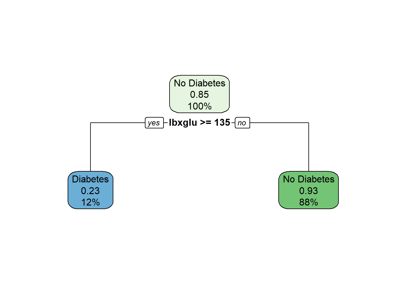

NULL

tree_prune$cptable

          CP nsplit rel error    xerror       xstd
1 0.41420118      0 1.0000000 1.0000000 0.07091587
2 0.02662722      1 0.5857988 0.6272189 0.05798252

str(tree_prune)

List of 15
 $ frame              :'data.frame':    3 obs. of  9 variables:
  ..$ var       : chr [1:3] "lbxglu" "<leaf>" "<leaf>"
  ..$ n         : int [1:3] 1126 132 994
  ..$ wt        : num [1:3] 1126 132 994
  ..$ dev       : num [1:3] 169 31 68
  ..$ yval      : num [1:3] 2 1 2
  ..$ complexity: num [1:3] 0.4142 0.0266 0.0118
  ..$ ncompete  : int [1:3] 4 0 0
  ..$ nsurrogate: int [1:3] 0 0 0
  ..$ yval2     : num [1:3, 1:6] 2 1 2 169 101 ...
  .. ..- attr(*, "dimnames")=List of 2
  .. .. ..$ : NULL
  .. .. ..$ : chr [1:6] "" "" "" "" ...
 $ where              : int [1:1126] 3 3 3 2 3 2 3 3 3 3 ...
 $ call               : language rpart(formula = diq010 ~ riagendr + ridageyr + ridreth1 + dmdeduc2 + dmdmartl +      indhhin2 + bmxbmi + lbxglu, | __truncated__ ...
 $ terms              :Classes 'terms', 'formula'  language diq010 ~ riagendr + ridageyr + ridreth1 + dmdeduc2 + dmdmartl + indhhin2 +      bmxbmi + lbxglu
  .. ..- attr(*, "variables")= language list(diq010, riagendr, ridageyr, ridreth1, dmdeduc2, dmdmartl, indhhin2,      bmxbmi, lbxglu)
  .. ..- attr(*, "factors")= int [1:9, 1:8] 0 1 0 0 0 0 0 0 0 0 ...
  .. .. ..- attr(*, "dimnames")=List of 2
  .. .. .. ..$ : chr [1:9] "diq010" "riagendr" "ridageyr" "ridreth1" ...
  .. .. .. ..$ : chr [1:8] "riagendr" "ridageyr" "ridreth1" "dmdeduc2" ...
  .. ..- attr(*, "term.labels")= chr [1:8] "riagendr" "ridageyr" "ridreth1" "dmdeduc2" ...
  .. ..- attr(*, "order")= int [1:8] 1 1 1 1 1 1 1 1
  .. ..- attr(*, "intercept")= int 1
  .. ..- attr(*, "response")= int 1
  .. ..- attr(*, ".Environment")=<environment: R_GlobalEnv> 
  .. ..- attr(*, "predvars")= language list(diq010, riagendr, ridageyr, ridreth1, dmdeduc2, dmdmartl, indhhin2,      bmxbmi, lbxglu)
  .. ..- attr(*, "dataClasses")= Named chr [1:9] "factor" "factor" "numeric" "factor" ...
  .. .. ..- attr(*, "names")= chr [1:9] "diq010" "riagendr" "ridageyr" "ridreth1" ...
 $ cptable            : num [1:2, 1:5] 0.4142 0.0266 0 1 1 ...
  ..- attr(*, "dimnames")=List of 2
  .. ..$ : chr [1:2] "1" "2"
  .. ..$ : chr [1:5] "CP" "nsplit" "rel error" "xerror" ...
 $ method             : chr "class"
 $ parms              :List of 3
  ..$ prior: num [1:2(1d)] 0.15 0.85
  .. ..- attr(*, "dimnames")=List of 1
  .. .. ..$ : chr [1:2] "1" "2"
  ..$ loss : num [1:2, 1:2] 0 1 1 0
  ..$ split: num 1
 $ control            :List of 9
  ..$ minsplit      : num 1
  ..$ minbucket     : num 1
  ..$ cp            : num 0.006
  ..$ maxcompete    : num 4
  ..$ maxsurrogate  : num 5
  ..$ usesurrogate  : num 2
  ..$ surrogatestyle: num 0
  ..$ maxdepth      : num 30
  ..$ xval          : num 10
 $ functions          :List of 3
  ..$ summary:function (yval, dev, wt, ylevel, digits)  
  ..$ print  :function (yval, ylevel, digits, nsmall)  
  ..$ text   :function (yval, dev, wt, ylevel, digits, n, use.n)  
 $ numresp            : int 4
 $ splits             : num [1:5, 1:5] 1126 1126 1126 1126 1126 ...
  ..- attr(*, "dimnames")=List of 2
  .. ..$ : chr [1:5] "lbxglu" "ridageyr" "bmxbmi" "dmdeduc2" ...
  .. ..$ : chr [1:5] "count" "ncat" "improve" "index" ...
 $ csplit             : int [1:2, 1:14] 1 1 3 1 3 1 3 1 3 3 ...
 $ variable.importance: Named num 113
  ..- attr(*, "names")= chr "lbxglu"
 $ y                  : int [1:1126] 2 2 2 1 2 2 2 2 2 2 ...
 $ ordered            : Named logi [1:8] FALSE FALSE FALSE FALSE FALSE FALSE ...
  ..- attr(*, "names")= chr [1:8] "riagendr" "ridageyr" "ridreth1" "dmdeduc2" ...
 - attr(*, "xlevels")=List of 5
  ..$ riagendr: chr [1:2] "Male" "Female"
  ..$ ridreth1: chr [1:5] "MexicanAmerican" "Other Hispanic" "Non-Hispanic White" "Non-Hispanic Black" ...
  ..$ dmdeduc2: chr [1:5] "Less than 9th grade" "Grades 9-11th" "High school graduate/GED" "Some college or AA degrees" ...
  ..$ dmdmartl: chr [1:6] "Married" "Widowed" "Divorced" "Separated" ...
  ..$ indhhin2: chr [1:14] "$0-$4,999" "$5,000-$9,999" "$10,000-$14,999" "$15,000-$19,999" ...
 - attr(*, "ylevels")= chr [1:2] "Diabetes" "No Diabetes"
 - attr(*, "class")= chr "rpart"

lbxglu_split_level <- tree_prune$splits['lbxglu','index']

\(~\)

21.8 Score Decision Tree Model on Training Set

\(~\)

21.8.1 Score Output Probabilities

y_hat_probs <- predict(tree_prune, train_set)

head(y_hat_probs)

     Diabetes No Diabetes
2  0.06841046   0.9315895
11 0.06841046   0.9315895
13 0.06841046   0.9315895
14 0.76515152   0.2348485
29 0.06841046   0.9315895
32 0.76515152   0.2348485

str(y_hat_probs)

 num [1:1126, 1:2] 0.0684 0.0684 0.0684 0.7652 0.0684 ...
 - attr(*, "dimnames")=List of 2
  ..$ : chr [1:1126] "2" "11" "13" "14" ...
  ..$ : chr [1:2] "Diabetes" "No Diabetes"

\(~\)

21.8.2 Score Output Class

y_hat_class <- predict(tree_prune, train_set, type ="class")

head(y_hat_class)

          2          11          13          14          29          32 
No Diabetes No Diabetes No Diabetes    Diabetes No Diabetes    Diabetes 
Levels: Diabetes No Diabetes

str(y_hat_class)

 Factor w/ 2 levels "Diabetes","No Diabetes": 2 2 2 1 2 1 2 2 2 2 ...
 - attr(*, "names")= chr [1:1126] "2" "11" "13" "14" ...

\(~\)

21.8.3 View Training Dataset with Scores

train.scored <- as_tibble(cbind(train_set, y_hat_probs, y_hat_class))

glimpse(train.scored)

Rows: 1,126
Columns: 13
$ seqn          <dbl> 83733, 83750, 83754, 83755, 83787, 83790, 83799, 83809, …
$ riagendr      <fct> Male, Male, Female, Male, Female, Male, Female, Female, …
$ ridageyr      <dbl> 53, 45, 67, 67, 68, 56, 37, 20, 24, 80, 39, 35, 40, 74, …
$ ridreth1      <fct> Non-Hispanic White, Other, Other Hispanic, Non-Hispanic …
$ dmdeduc2      <fct> High school graduate/GED, Grades 9-11th, College grad or…
$ dmdmartl      <fct> Divorced, Never married, Married, Widowed, Divorced, Mar…
$ indhhin2      <fct> "$15,000-$19,999", "$65,000-$74,999", "$25,000-$34,999",…
$ bmxbmi        <dbl> 30.8, 24.1, 43.7, 28.8, 33.5, 24.4, 25.5, 26.2, 26.9, 28…
$ diq010        <fct> No Diabetes, No Diabetes, No Diabetes, Diabetes, No Diab…
$ lbxglu        <dbl> 101, 84, 130, 284, 111, 397, 100, 94, 105, 119, 101, 97,…
$ Diabetes      <dbl> 0.06841046, 0.06841046, 0.06841046, 0.76515152, 0.068410…
$ `No Diabetes` <dbl> 0.9315895, 0.9315895, 0.9315895, 0.2348485, 0.9315895, 0…
$ y_hat_class   <fct> No Diabetes, No Diabetes, No Diabetes, Diabetes, No Diab…

\(~\)

21.9 Why was 135 chosen as the split value of `lbxglu`

The goal in some of these subsequent sections is to give some insight as to how the decision tree chooses to make the cut.

\(~\)

21.9.1 Compare Confusion Matrix and 2-by-2 Tables

library('caret')

cm_1 <- confusionMatrix( data = train.scored$y_hat_class,
                         reference = train.scored$diq010,
                         positive = 'Diabetes',
                         mode = "everything")

cm_1

Confusion Matrix and Statistics

             Reference
Prediction    Diabetes No Diabetes
  Diabetes         101          31
  No Diabetes       68         926
                                        
               Accuracy : 0.9121        
                 95% CI : (0.894, 0.928)
    No Information Rate : 0.8499        
    P-Value [Acc > NIR] : 2.918e-10     
                                        
                  Kappa : 0.6212        
                                        
 Mcnemar's Test P-Value : 0.0002967     
                                        
            Sensitivity : 0.5976        
            Specificity : 0.9676        
         Pos Pred Value : 0.7652        
         Neg Pred Value : 0.9316        
              Precision : 0.7652        
                 Recall : 0.5976        
                     F1 : 0.6711        
             Prevalence : 0.1501        
         Detection Rate : 0.0897        
   Detection Prevalence : 0.1172        
      Balanced Accuracy : 0.7826        
                                        
       'Positive' Class : Diabetes

str(cm_1)

List of 6
 $ positive: chr "Diabetes"
 $ table   : 'table' int [1:2, 1:2] 101 68 31 926
  ..- attr(*, "dimnames")=List of 2
  .. ..$ Prediction: chr [1:2] "Diabetes" "No Diabetes"
  .. ..$ Reference : chr [1:2] "Diabetes" "No Diabetes"
 $ overall : Named num [1:7] 0.912 0.621 0.894 0.928 0.85 ...
  ..- attr(*, "names")= chr [1:7] "Accuracy" "Kappa" "AccuracyLower" "AccuracyUpper" ...
 $ byClass : Named num [1:11] 0.598 0.968 0.765 0.932 0.765 ...
  ..- attr(*, "names")= chr [1:11] "Sensitivity" "Specificity" "Pos Pred Value" "Neg Pred Value" ...
 $ mode    : chr "everything"
 $ dots    : list()
 - attr(*, "class")= chr "confusionMatrix"

cm_1$table

             Reference
Prediction    Diabetes No Diabetes
  Diabetes         101          31
  No Diabetes       68         926

cm_1$byClass

         Sensitivity          Specificity       Pos Pred Value 
          0.59763314           0.96760711           0.76515152 
      Neg Pred Value            Precision               Recall 
          0.93158954           0.76515152           0.59763314 
                  F1           Prevalence       Detection Rate 
          0.67109635           0.15008881           0.08969805 
Detection Prevalence    Balanced Accuracy 
          0.11722913           0.78262012

table_1 <- table(train.scored$y_hat_class, train.scored$diq010)  

table_1

             
              Diabetes No Diabetes
  Diabetes         101          31
  No Diabetes       68         926

cm_1$table

             Reference
Prediction    Diabetes No Diabetes
  Diabetes         101          31
  No Diabetes       68         926

gplots::balloonplot(cm_1$table,
                    main ="Balloon Plot for lbxglu_flag by Diabetes \n Area is proportional to Freq.")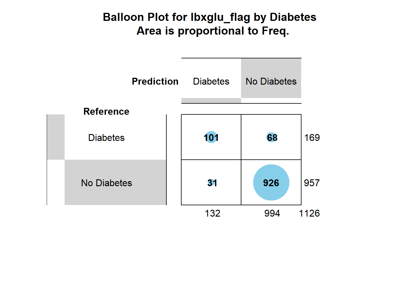

chisq.test(cm_1$table)$p.value

[1] 2.944895e-97

\(~\)

21.9.2 Programming a Confusion Matrix from a 2-by-2 Table

table_1 <- table(train.scored$y_hat_class, train.scored$diq010)

table_1

             
              Diabetes No Diabetes
  Diabetes         101          31
  No Diabetes       68         926

TP <- table_1[1,1]
FP <- table_1[1,2]
FN <- table_1[2,1]
TN <- table_1[2,2]

TPR = TP / (TP+FN)
TNR = TN / (TN+FP)

PPV = TP / (TP+FP)
NPV = TN / (TN+FN)

ACC = (TP+TN)/(TP+TN+FP+FN)

F1 = 2/((1/TPR) + (1/PPV))

\(~\)

21.9.2.1 Check our work

cm_1$byClass['Sensitivity'] - TPR

Sensitivity 
          0

cm_1$byClass['Specificity'] - TNR

Specificity 
          0

cm_1$byClass['Pos Pred Value'] - PPV

Pos Pred Value 
 -1.110223e-16

cm_1$overall['Accuracy'] - ACC

Accuracy 
       0

cm_1$byClass['F1'] - F1

F1 
 0

\(~\)

21.10 Decision Tree - Choosing the Cut Point

The goal in some of these subsequent sections is to give some insight as to how the decision tree chooses to make the cut.

This function, will:

Take in a value for lbxglu
If the recorded value for lbxglu is greater than or equal to the input value, then the record is flagged with lbxglu_over_value, otherwise it is flagged with lbxglu_under_value
A 2-by-2 table is then created to mirror the confusion matrix of that decision
Metrics are reported and returned for that decision:

lbxglu_value_chisq <- function(my_value, return_table=0){ 
  require('tidyverse')
  
  dt <- train_set %>%
          mutate(lbxglu_flag = ifelse(lbxglu >= my_value,"lbxglu_over_value","lbxglu_under_value") ) 
    
  table_1 <- table(dt$lbxglu_flag , dt$diq010)
  
  if(return_table ==1 ){return(table_1)}
  
  TP <- table_1[1,1]
  FP <- table_1[1,2]
  FN <- table_1[2,1]
  TN <- table_1[2,2]

  TPR = TP / (TP+FN)
  TNR = TN / (TN+FP)

  PPV = TP / (TP+FP)
  NPV = TN / (TN+FN)

  ACC = (TP+TN)/(TP+TN+FP+FN)

  F1 = 2/((1/TPR) + (1/PPV))
  
  # GINI AND INFORMATION
    base_prob <-table(dt$lbxglu_flag)/length(dt$lbxglu_flag)
    crosstab <- table(dt$diq010, dt$lbxglu_flag)
    crossprob <- prop.table(crosstab,2)

  # GINI
    No_Node_Gini <- 1-sum(crossprob[,1]**2)
    Yes_Node_Gini <- 1-sum(crossprob[,2]**2)
    GINI <- sum(base_prob * c(No_Node_Gini,Yes_Node_Gini))

  # INFORMATION
    No_Col <- crossprob[crossprob[,1]>0,1]
    Yes_Col <- crossprob[crossprob[,2]>0,2]
    No_Node_Info <- -sum(No_Col*log(No_Col,2))
    Yes_Node_Info <- -sum(Yes_Col*log(Yes_Col,2))
    Information <- sum(base_prob * c(No_Node_Info,Yes_Node_Info))
  
  table_1_chisq_pvalue <- tibble::enframe(chisq.test(table_1)$p.value) %>%
    rename(chisq_p_value = value) %>%
    select(-name) %>%
    mutate(lbxglu_value = my_value) %>%
    select(lbxglu_value, chisq_p_value) %>%
    mutate( TP = TP ) %>%
    mutate( FP = FP ) %>%
    mutate( FN = FN ) %>%
    mutate( TN = TN ) %>%  
    mutate( PPV = PPV ) %>%
    mutate( TPR = TPR ) %>%
    mutate( ACC = ACC ) %>%
    mutate( F1 = F1 ) %>%
    mutate( GINI = GINI ) %>%
    mutate(Information = Information)

  return( table_1_chisq_pvalue )
}

\(~\)

21.10.1 Test `lbxglu_value_chisq` Function

Let’s test our function!

lbxglu_split_level

[1] 135

lbxglu_value_chisq(lbxglu_split_level, return_table=1)

                    
                     Diabetes No Diabetes
  lbxglu_over_value       101          31
  lbxglu_under_value       68         926

cm_1$table

             Reference
Prediction    Diabetes No Diabetes
  Diabetes         101          31
  No Diabetes       68         926

glimpse(lbxglu_value_chisq(lbxglu_split_level))

Rows: 1
Columns: 12
$ lbxglu_value  <dbl> 135
$ chisq_p_value <dbl> 2.944895e-97
$ TP            <int> 101
$ FP            <int> 31
$ FN            <int> 68
$ TN            <int> 926
$ PPV           <dbl> 0.7651515
$ TPR           <dbl> 0.5976331
$ ACC           <dbl> 0.9120782
$ F1            <dbl> 0.6710963
$ GINI          <dbl> 0.1546497
$ Information   <dbl> 0.4099506

\(~\)

21.11 Find Ranges

Now let’s find the ranges of values for which to apply our function:

range_lbxglu_by_diq010 <- train_set %>% 
  group_by(diq010) %>% 
  summarise(lbxglu_min = min(lbxglu,na.rm=TRUE) , lbxglu_max = max(lbxglu,na.rm=TRUE) )

range_lbxglu_by_diq010

# A tibble: 2 × 3
  diq010      lbxglu_min lbxglu_max
  <fct>            <dbl>      <dbl>
1 Diabetes            50        479
2 No Diabetes         64        397

my_min <- min(range_lbxglu_by_diq010$lbxglu_min) +1
my_min

[1] 51

# note anything less than `my_min` does not produce a 2x2 table:

lbxglu_value_chisq(my_min-1, return_table=1)

                   
                    Diabetes No Diabetes
  lbxglu_over_value      169         957

lbxglu_value_chisq(my_min, return_table=1)

                    
                     Diabetes No Diabetes
  lbxglu_over_value       168         957
  lbxglu_under_value        1           0

my_max <- max(range_lbxglu_by_diq010$lbxglu_max)
my_max

[1] 479

# note anything more than `my_max` does not produce a 2x2 table:
lbxglu_value_chisq(my_max, return_table=1)

                    
                     Diabetes No Diabetes
  lbxglu_over_value         1           0
  lbxglu_under_value      168         957

lbxglu_value_chisq(my_max+1, return_table=1)

                    
                     Diabetes No Diabetes
  lbxglu_under_value      169         957

# so the range of values are:
my_list <- my_min:my_max
my_list

  [1]  51  52  53  54  55  56  57  58  59  60  61  62  63  64  65  66  67  68
 [19]  69  70  71  72  73  74  75  76  77  78  79  80  81  82  83  84  85  86
 [37]  87  88  89  90  91  92  93  94  95  96  97  98  99 100 101 102 103 104
 [55] 105 106 107 108 109 110 111 112 113 114 115 116 117 118 119 120 121 122
 [73] 123 124 125 126 127 128 129 130 131 132 133 134 135 136 137 138 139 140
 [91] 141 142 143 144 145 146 147 148 149 150 151 152 153 154 155 156 157 158
[109] 159 160 161 162 163 164 165 166 167 168 169 170 171 172 173 174 175 176
[127] 177 178 179 180 181 182 183 184 185 186 187 188 189 190 191 192 193 194
[145] 195 196 197 198 199 200 201 202 203 204 205 206 207 208 209 210 211 212
[163] 213 214 215 216 217 218 219 220 221 222 223 224 225 226 227 228 229 230
[181] 231 232 233 234 235 236 237 238 239 240 241 242 243 244 245 246 247 248
[199] 249 250 251 252 253 254 255 256 257 258 259 260 261 262 263 264 265 266
[217] 267 268 269 270 271 272 273 274 275 276 277 278 279 280 281 282 283 284
[235] 285 286 287 288 289 290 291 292 293 294 295 296 297 298 299 300 301 302
[253] 303 304 305 306 307 308 309 310 311 312 313 314 315 316 317 318 319 320
[271] 321 322 323 324 325 326 327 328 329 330 331 332 333 334 335 336 337 338
[289] 339 340 341 342 343 344 345 346 347 348 349 350 351 352 353 354 355 356
[307] 357 358 359 360 361 362 363 364 365 366 367 368 369 370 371 372 373 374
[325] 375 376 377 378 379 380 381 382 383 384 385 386 387 388 389 390 391 392
[343] 393 394 395 396 397 398 399 400 401 402 403 404 405 406 407 408 409 410
[361] 411 412 413 414 415 416 417 418 419 420 421 422 423 424 425 426 427 428
[379] 429 430 431 432 433 434 435 436 437 438 439 440 441 442 443 444 445 446
[397] 447 448 449 450 451 452 453 454 455 456 457 458 459 460 461 462 463 464
[415] 465 466 467 468 469 470 471 472 473 474 475 476 477 478 479

\(~\)

21.12 Apply Function

Now we apply our function lbxglu_value_chisq to the range my_list

chi_square_lbxglu_value <- purrr::map_dfr(my_list, lbxglu_value_chisq) 

glimpse(chi_square_lbxglu_value)

Rows: 429
Columns: 12
$ lbxglu_value  <int> 51, 52, 53, 54, 55, 56, 57, 58, 59, 60, 61, 62, 63, 64, …
$ chisq_p_value <dbl> 0.3270151, 0.3270151, 0.3270151, 0.3270151, 0.3270151, 0…
$ TP            <int> 168, 168, 168, 168, 168, 168, 168, 168, 168, 168, 168, 1…
$ FP            <int> 957, 957, 957, 957, 957, 957, 957, 957, 957, 957, 957, 9…
$ FN            <int> 1, 1, 1, 1, 1, 1, 1, 1, 1, 1, 1, 1, 1, 1, 1, 1, 1, 1, 1,…
$ TN            <int> 0, 0, 0, 0, 0, 0, 0, 0, 0, 0, 0, 0, 0, 0, 1, 2, 2, 2, 2,…
$ PPV           <dbl> 0.1493333, 0.1493333, 0.1493333, 0.1493333, 0.1493333, 0…
$ TPR           <dbl> 0.9940828, 0.9940828, 0.9940828, 0.9940828, 0.9940828, 0…
$ ACC           <dbl> 0.1492007, 0.1492007, 0.1492007, 0.1492007, 0.1492007, 0…
$ F1            <dbl> 0.2596600, 0.2596600, 0.2596600, 0.2596600, 0.2596600, 0…
$ GINI          <dbl> 0.2538401, 0.2538401, 0.2538401, 0.2538401, 0.2538401, 0…
$ Information   <dbl> 0.6076293, 0.6076293, 0.6076293, 0.6076293, 0.6076293, 0…

\(~\)

21.12.1 Sort Review Results

Let’s review the Results by sorting them with respect to different metrics:

chi_square_lbxglu_value %>% arrange(chisq_p_value)

# A tibble: 429 × 12
   lbxglu_value chisq_p_value    TP    FP    FN    TN   PPV   TPR   ACC    F1
          <int>         <dbl> <int> <int> <int> <int> <dbl> <dbl> <dbl> <dbl>
 1          135      2.94e-97   101    31    68   926 0.765 0.598 0.912 0.671
 2          136      2.94e-97   101    31    68   926 0.765 0.598 0.912 0.671
 3          141      3.60e-97    95    23    74   934 0.805 0.562 0.914 0.662
 4          134      4.00e-97   103    34    66   923 0.752 0.609 0.911 0.673
 5          133      1.26e-96   104    36    65   921 0.743 0.615 0.910 0.673
 6          139      2.01e-96    96    25    73   932 0.793 0.568 0.913 0.662
 7          145      2.68e-96    92    20    77   937 0.821 0.544 0.914 0.655
 8          138      4.24e-96    98    28    71   929 0.778 0.580 0.912 0.664
 9          140      4.29e-96    95    24    74   933 0.798 0.562 0.913 0.660
10          142      8.92e-96    94    23    75   934 0.803 0.556 0.913 0.657
# ℹ 419 more rows
# ℹ 2 more variables: GINI <dbl>, Information <dbl>

chi_square_lbxglu_value %>% arrange(GINI)

# A tibble: 429 × 12
   lbxglu_value chisq_p_value    TP    FP    FN    TN   PPV   TPR   ACC    F1
          <int>         <dbl> <int> <int> <int> <int> <dbl> <dbl> <dbl> <dbl>
 1          135      2.94e-97   101    31    68   926 0.765 0.598 0.912 0.671
 2          136      2.94e-97   101    31    68   926 0.765 0.598 0.912 0.671
 3          141      3.60e-97    95    23    74   934 0.805 0.562 0.914 0.662
 4          134      4.00e-97   103    34    66   923 0.752 0.609 0.911 0.673
 5          133      1.26e-96   104    36    65   921 0.743 0.615 0.910 0.673
 6          139      2.01e-96    96    25    73   932 0.793 0.568 0.913 0.662
 7          145      2.68e-96    92    20    77   937 0.821 0.544 0.914 0.655
 8          140      4.29e-96    95    24    74   933 0.798 0.562 0.913 0.660
 9          138      4.24e-96    98    28    71   929 0.778 0.580 0.912 0.664
10          142      8.92e-96    94    23    75   934 0.803 0.556 0.913 0.657
# ℹ 419 more rows
# ℹ 2 more variables: GINI <dbl>, Information <dbl>

chi_square_lbxglu_value %>% arrange(Information)

# A tibble: 429 × 12
   lbxglu_value chisq_p_value    TP    FP    FN    TN   PPV   TPR   ACC    F1
          <int>         <dbl> <int> <int> <int> <int> <dbl> <dbl> <dbl> <dbl>
 1          122      1.10e-90   120    71    49   886 0.628 0.710 0.893 0.667
 2          134      4.00e-97   103    34    66   923 0.752 0.609 0.911 0.673
 3          133      1.26e-96   104    36    65   921 0.743 0.615 0.910 0.673
 4          135      2.94e-97   101    31    68   926 0.765 0.598 0.912 0.671
 5          136      2.94e-97   101    31    68   926 0.765 0.598 0.912 0.671
 6          130      7.29e-95   106    41    63   916 0.721 0.627 0.908 0.671
 7          123      3.54e-90   117    66    52   891 0.639 0.692 0.895 0.665
 8          121      4.26e-88   121    77    48   880 0.611 0.716 0.889 0.659
 9          125      3.25e-91   114    59    55   898 0.659 0.675 0.899 0.667
10          131      2.21e-94   105    40    64   917 0.724 0.621 0.908 0.669
# ℹ 419 more rows
# ℹ 2 more variables: GINI <dbl>, Information <dbl>

chi_square_lbxglu_value %>% arrange(-ACC)

# A tibble: 429 × 12
   lbxglu_value chisq_p_value    TP    FP    FN    TN   PPV   TPR   ACC    F1
          <int>         <dbl> <int> <int> <int> <int> <dbl> <dbl> <dbl> <dbl>
 1          141      3.60e-97    95    23    74   934 0.805 0.562 0.914 0.662
 2          145      2.68e-96    92    20    77   937 0.821 0.544 0.914 0.655
 3          139      2.01e-96    96    25    73   932 0.793 0.568 0.913 0.662
 4          140      4.29e-96    95    24    74   933 0.798 0.562 0.913 0.660
 5          142      8.92e-96    94    23    75   934 0.803 0.556 0.913 0.657
 6          146      6.67e-95    91    20    78   937 0.820 0.538 0.913 0.65 
 7          147      1.22e-94    90    19    79   938 0.826 0.533 0.913 0.647
 8          149      3.68e-94    88    17    81   940 0.838 0.521 0.913 0.642
 9          152      1.43e-93    85    14    84   943 0.859 0.503 0.913 0.634
10          153      1.43e-93    85    14    84   943 0.859 0.503 0.913 0.634
# ℹ 419 more rows
# ℹ 2 more variables: GINI <dbl>, Information <dbl>

chi_square_lbxglu_value %>% arrange(-PPV)

# A tibble: 429 × 12
   lbxglu_value chisq_p_value    TP    FP    FN    TN   PPV    TPR   ACC     F1
          <int>         <dbl> <int> <int> <int> <int> <dbl>  <dbl> <dbl>  <dbl>
 1          398    0.00000253     5     0   164   957     1 0.0296 0.854 0.0575
 2          399    0.00000253     5     0   164   957     1 0.0296 0.854 0.0575
 3          400    0.00000253     5     0   164   957     1 0.0296 0.854 0.0575
 4          401    0.00000253     5     0   164   957     1 0.0296 0.854 0.0575
 5          402    0.00000253     5     0   164   957     1 0.0296 0.854 0.0575
 6          403    0.00000253     5     0   164   957     1 0.0296 0.854 0.0575
 7          404    0.00000253     5     0   164   957     1 0.0296 0.854 0.0575
 8          405    0.00000253     5     0   164   957     1 0.0296 0.854 0.0575
 9          406    0.00000253     5     0   164   957     1 0.0296 0.854 0.0575
10          407    0.00000253     5     0   164   957     1 0.0296 0.854 0.0575
# ℹ 419 more rows
# ℹ 2 more variables: GINI <dbl>, Information <dbl>

chi_square_lbxglu_value %>% arrange(-F1)

# A tibble: 429 × 12
   lbxglu_value chisq_p_value    TP    FP    FN    TN   PPV   TPR   ACC    F1
          <int>         <dbl> <int> <int> <int> <int> <dbl> <dbl> <dbl> <dbl>
 1          134      4.00e-97   103    34    66   923 0.752 0.609 0.911 0.673
 2          133      1.26e-96   104    36    65   921 0.743 0.615 0.910 0.673
 3          135      2.94e-97   101    31    68   926 0.765 0.598 0.912 0.671
 4          136      2.94e-97   101    31    68   926 0.765 0.598 0.912 0.671
 5          130      7.29e-95   106    41    63   916 0.721 0.627 0.908 0.671
 6          131      2.21e-94   105    40    64   917 0.724 0.621 0.908 0.669
 7          122      1.10e-90   120    71    49   886 0.628 0.710 0.893 0.667
 8          125      3.25e-91   114    59    55   898 0.659 0.675 0.899 0.667
 9          129      3.82e-93   106    43    63   914 0.711 0.627 0.906 0.667
10          132      6.57e-94   104    39    65   918 0.727 0.615 0.908 0.667
# ℹ 419 more rows
# ℹ 2 more variables: GINI <dbl>, Information <dbl>

\(~\)

21.13 Plot Results

Let’s Plot Our Results

glimpse(chi_square_lbxglu_value)

Rows: 429
Columns: 12
$ lbxglu_value  <int> 51, 52, 53, 54, 55, 56, 57, 58, 59, 60, 61, 62, 63, 64, …
$ chisq_p_value <dbl> 0.3270151, 0.3270151, 0.3270151, 0.3270151, 0.3270151, 0…
$ TP            <int> 168, 168, 168, 168, 168, 168, 168, 168, 168, 168, 168, 1…
$ FP            <int> 957, 957, 957, 957, 957, 957, 957, 957, 957, 957, 957, 9…
$ FN            <int> 1, 1, 1, 1, 1, 1, 1, 1, 1, 1, 1, 1, 1, 1, 1, 1, 1, 1, 1,…
$ TN            <int> 0, 0, 0, 0, 0, 0, 0, 0, 0, 0, 0, 0, 0, 0, 1, 2, 2, 2, 2,…
$ PPV           <dbl> 0.1493333, 0.1493333, 0.1493333, 0.1493333, 0.1493333, 0…
$ TPR           <dbl> 0.9940828, 0.9940828, 0.9940828, 0.9940828, 0.9940828, 0…
$ ACC           <dbl> 0.1492007, 0.1492007, 0.1492007, 0.1492007, 0.1492007, 0…
$ F1            <dbl> 0.2596600, 0.2596600, 0.2596600, 0.2596600, 0.2596600, 0…
$ GINI          <dbl> 0.2538401, 0.2538401, 0.2538401, 0.2538401, 0.2538401, 0…
$ Information   <dbl> 0.6076293, 0.6076293, 0.6076293, 0.6076293, 0.6076293, 0…

chi_square_lbxglu_value.ggplot_data <- chi_square_lbxglu_value %>% 
  select(lbxglu_value, chisq_p_value, PPV, TPR, ACC, F1, GINI, Information) %>%
  gather(-lbxglu_value, key="stat_test", value="Value")

glimpse(chi_square_lbxglu_value.ggplot_data)

Rows: 3,003
Columns: 3
$ lbxglu_value <int> 51, 52, 53, 54, 55, 56, 57, 58, 59, 60, 61, 62, 63, 64, 6…
$ stat_test    <chr> "chisq_p_value", "chisq_p_value", "chisq_p_value", "chisq…
$ Value        <dbl> 0.3270151, 0.3270151, 0.3270151, 0.3270151, 0.3270151, 0.…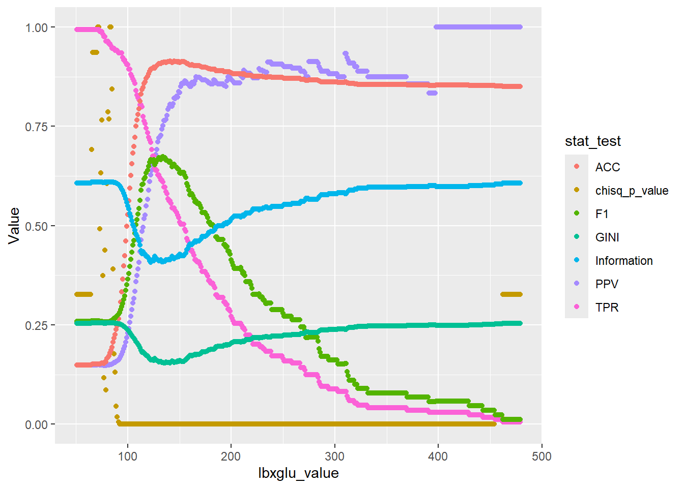

library('ggplot2')

plot_1 <- chi_square_lbxglu_value.ggplot_data %>%
  ggplot(aes(x=lbxglu_value, y=Value, color=stat_test)) +
  geom_point() 

plot_1

\(~\)

Now let’s add in the lbxglu_split_level from the decision tree:

plot_1 + geom_vline(xintercept = lbxglu_split_level)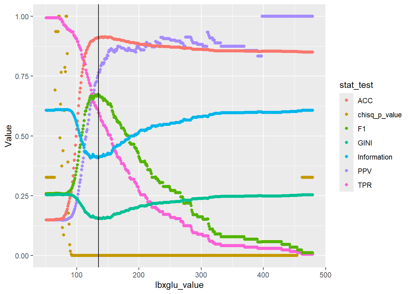

\(~\)

While some metrics such as PPV continue to impove, we can see that the F1 score is maximized around lbxglu_split_level.

Typically, when fitting a decision tree the GINI or Information is used to determine the splits and the order of the splits.

Hopefully, this gives some indication of how why split value lbxglu_split_level is equal to 135.

\(~\)

22 Score The Test Data

Now that we have a better understanding of what the decision tree model is doing, we will score the test data:

test <- diab_pop.no_na_vals.test

test.prune.y_hat_probs <- predict(tree_prune, test)
test.prune.y_hat_class <- predict(tree_prune, test, type ="class")

test.prune_scored <- as_tibble(cbind(test, test.prune.y_hat_probs, test.prune.y_hat_class))

glimpse(test.prune_scored)

Rows: 750
Columns: 13
$ seqn                   <dbl> 83734, 83737, 83757, 83761, 83789, 83820, 83822…
$ riagendr               <fct> Male, Female, Female, Female, Male, Male, Femal…
$ ridageyr               <dbl> 78, 72, 57, 24, 66, 70, 20, 29, 69, 71, 37, 49,…
$ ridreth1               <fct> Non-Hispanic White, MexicanAmerican, Other Hisp…
$ dmdeduc2               <fct> High school graduate/GED, Grades 9-11th, Less t…
$ dmdmartl               <fct> Married, Separated, Separated, Never married, L…
$ indhhin2               <fct> "$20,000-$24,999", "$75,000-$99,999", "$20,000-…
$ bmxbmi                 <dbl> 28.8, 28.6, 35.4, 25.3, 34.0, 27.0, 22.2, 29.7,…
$ diq010                 <fct> Diabetes, No Diabetes, Diabetes, No Diabetes, N…
$ lbxglu                 <dbl> 84, 107, 398, 95, 113, 94, 80, 102, 105, 76, 79…
$ Diabetes               <dbl> 0.06841046, 0.06841046, 0.76515152, 0.06841046,…
$ `No Diabetes`          <dbl> 0.9315895, 0.9315895, 0.2348485, 0.9315895, 0.9…
$ test.prune.y_hat_class <fct> No Diabetes, No Diabetes, Diabetes, No Diabetes…

prune_cm_test <- confusionMatrix(data = test.prune_scored$test.prune.y_hat_class,
                           reference = test.prune_scored$diq010,
                           positive = 'Diabetes',
                           mode = "everything")

prune_cm_test

Confusion Matrix and Statistics

             Reference
Prediction    Diabetes No Diabetes
  Diabetes          63          21
  No Diabetes       49         617
                                          
               Accuracy : 0.9067          
                 95% CI : (0.8836, 0.9265)
    No Information Rate : 0.8507          
    P-Value [Acc > NIR] : 3.387e-06       
                                          
                  Kappa : 0.5904          
                                          
 Mcnemar's Test P-Value : 0.00125         
                                          
            Sensitivity : 0.5625          
            Specificity : 0.9671          
         Pos Pred Value : 0.7500          
         Neg Pred Value : 0.9264          
              Precision : 0.7500          
                 Recall : 0.5625          
                     F1 : 0.6429          
             Prevalence : 0.1493          
         Detection Rate : 0.0840          
   Detection Prevalence : 0.1120          
      Balanced Accuracy : 0.7648          
                                          
       'Positive' Class : Diabetes

\(~\)

22.1 Use `yardstick` for Model Metrics

install_if_not('yardstick')

[1] "the package 'yardstick' is already installed"

library('yardstick')


Attaching package: 'yardstick'

The following objects are masked from 'package:caret':

    precision, recall, sensitivity, specificity

The following object is masked from 'package:readr':

    spec

cm_2 <- test.prune_scored %>% 
  conf_mat(truth = diq010, estimate = test.prune.y_hat_class )

summary(cm_2)

# A tibble: 13 × 3
   .metric              .estimator .estimate
   <chr>                <chr>          <dbl>
 1 accuracy             binary         0.907
 2 kap                  binary         0.590
 3 sens                 binary         0.562
 4 spec                 binary         0.967
 5 ppv                  binary         0.75 
 6 npv                  binary         0.926
 7 mcc                  binary         0.599
 8 j_index              binary         0.530
 9 bal_accuracy         binary         0.765
10 detection_prevalence binary         0.112
11 precision            binary         0.75 
12 recall               binary         0.562
13 f_meas               binary         0.643

accuracy_val <- (summary(cm_2) %>% filter(.metric == 'accuracy'))$.estimate

accuracy_val

[1] 0.9066667

autoplot(cm_2)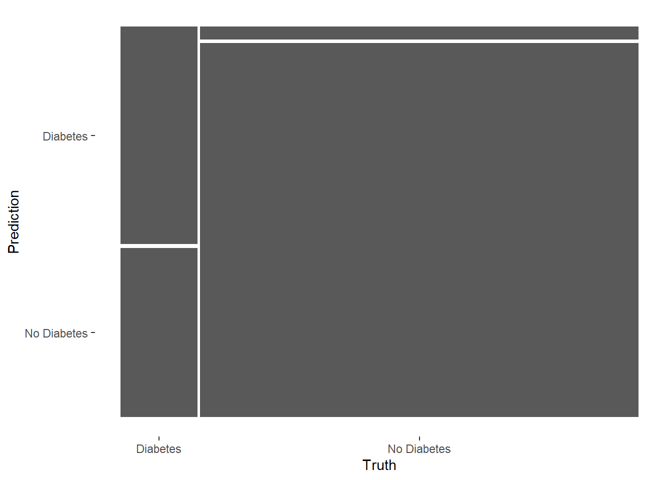

autoplot(cm_2, type = "heatmap")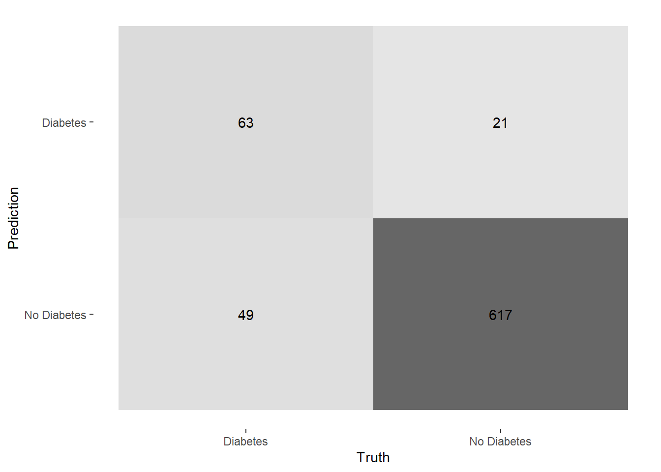

str(cm_2)

List of 1
 $ table: 'table' num [1:2, 1:2] 63 49 21 617
  ..- attr(*, "dimnames")=List of 2
  .. ..$ Prediction: chr [1:2] "Diabetes" "No Diabetes"
  .. ..$ Truth     : chr [1:2] "Diabetes" "No Diabetes"
 - attr(*, "class")= chr "conf_mat"

gplots::balloonplot(cm_2$table,
                    main ="Balloon Plot Confusion Matrix for Pruned Model \n Area is proportional to Freq.")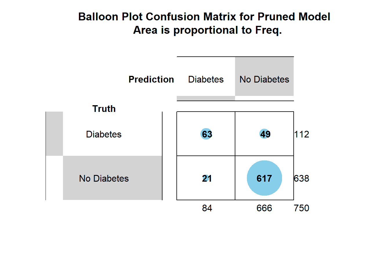

\(~\)

22.2 ROC Curve

metrics.prune <- test.prune_scored %>% 
  metrics(truth=diq010, test.prune.y_hat_class)

metrics.prune

# A tibble: 2 × 3
  .metric  .estimator .estimate
  <chr>    <chr>          <dbl>
1 accuracy binary         0.907
2 kap      binary         0.590

roc_auc.prune <- test.prune_scored %>%
  roc_auc(truth=diq010, Diabetes)

roc_auc.prune

# A tibble: 1 × 3
  .metric .estimator .estimate
  <chr>   <chr>          <dbl>
1 roc_auc binary         0.765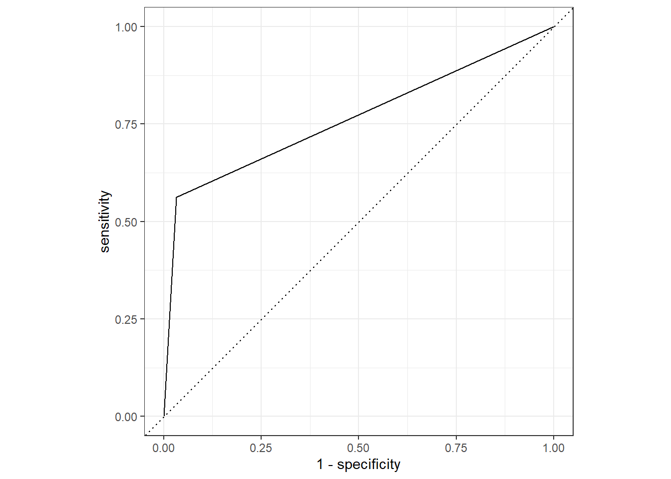

test_prune_roc <- test.prune_scored %>% 
  roc_curve(truth=diq010, Diabetes) 

autoplot(test_prune_roc)

plot_1 <- test_prune_roc %>%
  ggplot(aes(x = 1 - specificity, y = sensitivity)) +
  geom_path() +
  geom_abline(lty = 3) +
  coord_equal() +
  theme_bw()

plot_1

autoplot(test_prune_roc) + 
  labs( title = "ROC Curve - Pruned Model",
        caption = paste0("Area Under ROC Curve : ", round(roc_auc.prune$.estimate,3) )  ) +
  theme( plot.title = element_text(size = 18) , 
         plot.caption = element_text(size = 12))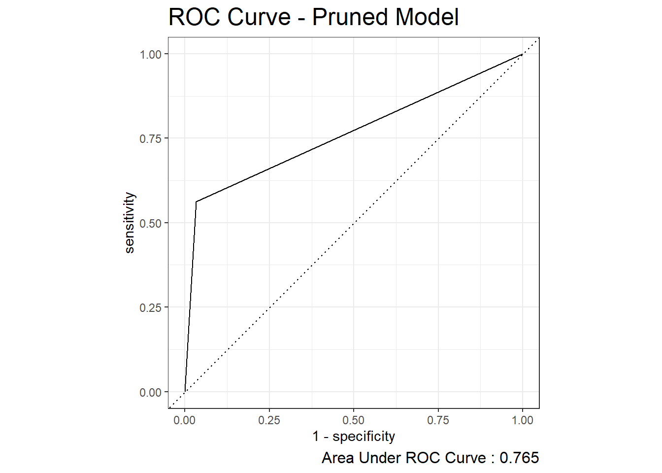

\(~\)

22.3 Precision Recall Curve

test_prune_pr_auc <- test.prune_scored %>%
  pr_auc(truth=diq010, Diabetes)

test_prune_pr_auc

# A tibble: 1 × 3
  .metric .estimator .estimate
  <chr>   <chr>          <dbl>
1 pr_auc  binary         0.689

test_prune_precision_recall <- test.prune_scored %>% 
  pr_curve(truth=diq010, Diabetes) 
 
autoplot(test_prune_precision_recall) + 
  labs( title = "Precision Recall Curve - Pruned Model",
        caption = paste0("Area Under Precision Recall Curve : ", round(test_prune_pr_auc$.estimate,3) )  ) +
  theme( plot.title = element_text(size = 18) , 
         plot.caption = element_text(size = 12))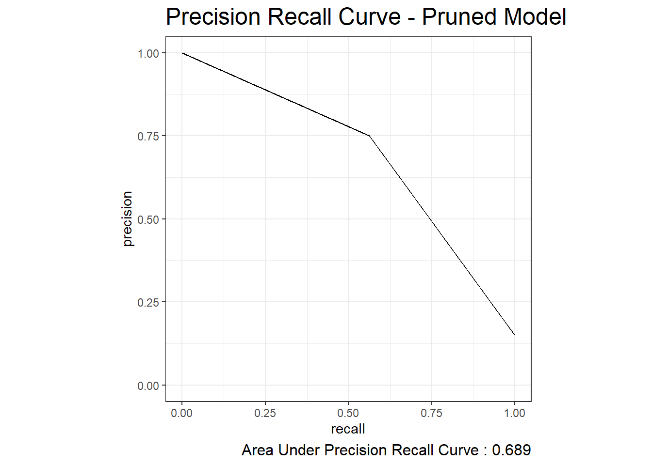

\(~\)

22.4 Lift Curve

test_prune_lift <- test.prune_scored %>% 
  lift_curve(truth=diq010, Diabetes) 
 
autoplot(test_prune_lift) + 
  labs( title = "Lift Curve - Pruned Model") +
  theme(plot.title = element_text(size = 18))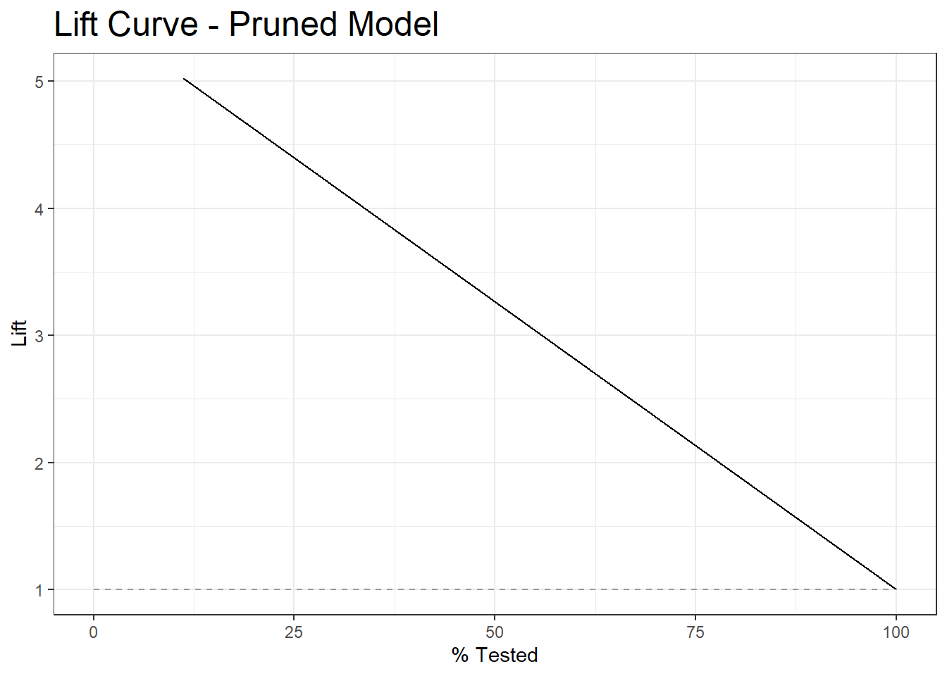

\(~\)

22.5 Gain Curve

test_prune_gain <- test.prune_scored %>% 
  gain_curve(truth=diq010, Diabetes) 
 
autoplot(test_prune_gain) + 
  labs( title = "Gain Curve - Pruned Model") +
  theme(plot.title = element_text(size = 18))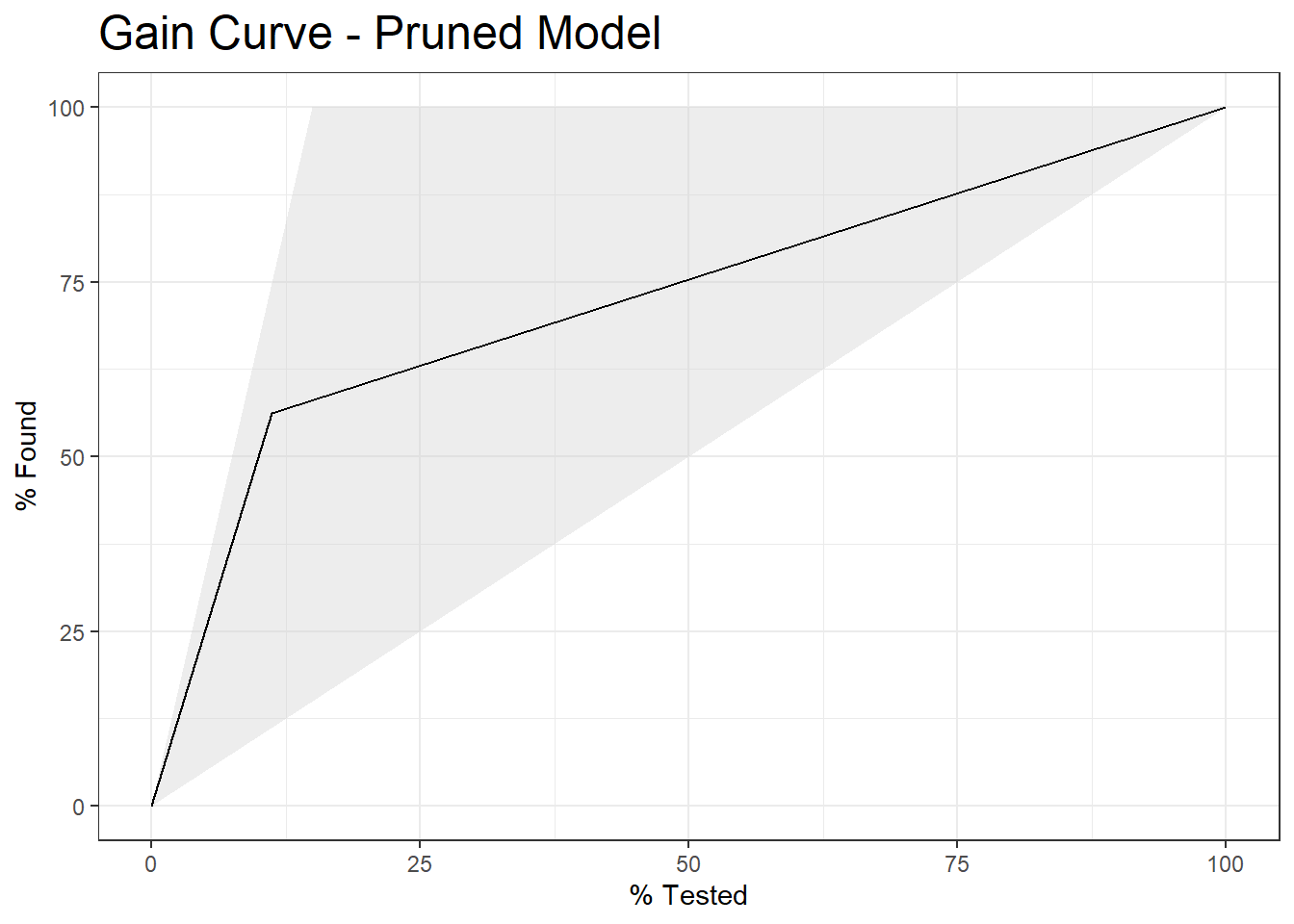

\(~\)

22.6 Comparing Models

A common task will be to compare the effectiveness of two models.

In this case, we will compare our pruned model to our origional model.

# pruned model
glimpse(test.prune_scored)

Rows: 750
Columns: 13
$ seqn                   <dbl> 83734, 83737, 83757, 83761, 83789, 83820, 83822…
$ riagendr               <fct> Male, Female, Female, Female, Male, Male, Femal…
$ ridageyr               <dbl> 78, 72, 57, 24, 66, 70, 20, 29, 69, 71, 37, 49,…
$ ridreth1               <fct> Non-Hispanic White, MexicanAmerican, Other Hisp…
$ dmdeduc2               <fct> High school graduate/GED, Grades 9-11th, Less t…
$ dmdmartl               <fct> Married, Separated, Separated, Never married, L…
$ indhhin2               <fct> "$20,000-$24,999", "$75,000-$99,999", "$20,000-…
$ bmxbmi                 <dbl> 28.8, 28.6, 35.4, 25.3, 34.0, 27.0, 22.2, 29.7,…
$ diq010                 <fct> Diabetes, No Diabetes, Diabetes, No Diabetes, N…
$ lbxglu                 <dbl> 84, 107, 398, 95, 113, 94, 80, 102, 105, 76, 79…
$ Diabetes               <dbl> 0.06841046, 0.06841046, 0.76515152, 0.06841046,…
$ `No Diabetes`          <dbl> 0.9315895, 0.9315895, 0.2348485, 0.9315895, 0.9…
$ test.prune.y_hat_class <fct> No Diabetes, No Diabetes, Diabetes, No Diabetes…

test.prune_scored_sel <- test.prune_scored %>% 
  select(seqn,diq010, Diabetes, test.prune.y_hat_class) %>%
  rename(pred_prob = Diabetes) %>%
  rename(pred_class = test.prune.y_hat_class) %>%
  mutate(model_type = 'prune')

# Score the Original Model on Test Data
test.y_hat_probs <- predict(tree_1, test)
test.y_hat_class <- predict(tree_1, test, type ="class")

test.scored <- as_tibble(cbind(test, test.y_hat_probs, test.y_hat_class))

test.scored_sel <- test.scored %>% 
  select(seqn,diq010, Diabetes, test.y_hat_class) %>%
  rename(pred_prob = Diabetes) %>%
  rename(pred_class = test.y_hat_class) %>%
  mutate(model_type = 'not_pruned')  

stacked_dfs <- rbind(test.prune_scored_sel, test.scored_sel) 

glimpse(stacked_dfs)

Rows: 1,500
Columns: 5
$ seqn       <dbl> 83734, 83737, 83757, 83761, 83789, 83820, 83822, 83823, 838…
$ diq010     <fct> Diabetes, No Diabetes, Diabetes, No Diabetes, No Diabetes, …
$ pred_prob  <dbl> 0.06841046, 0.06841046, 0.76515152, 0.06841046, 0.06841046,…
$ pred_class <fct> No Diabetes, No Diabetes, Diabetes, No Diabetes, No Diabete…
$ model_type <chr> "prune", "prune", "prune", "prune", "prune", "prune", "prun…

22.7 Compare Model Metrics

cm_compare <- stacked_dfs %>% 
  group_by(model_type) %>%
  conf_mat(truth = diq010, estimate = pred_class ) 

cm_compare

# A tibble: 2 × 2
  model_type conf_mat  
  <chr>      <list>    
1 not_pruned <conf_mat>
2 prune      <conf_mat>

cm_compare$conf_mat

[[1]]
             Truth
Prediction    Diabetes No Diabetes
  Diabetes          60          32
  No Diabetes       52         606

[[2]]
             Truth
Prediction    Diabetes No Diabetes
  Diabetes          63          21
  No Diabetes       49         617

(cm_compare %>% filter(model_type == 'prune'))$conf_mat

[[1]]
             Truth
Prediction    Diabetes No Diabetes
  Diabetes          63          21
  No Diabetes       49         617

prune_cm <- (cm_compare %>% filter(model_type == 'prune'))$conf_mat[[1]]
prune_cm

             Truth
Prediction    Diabetes No Diabetes
  Diabetes          63          21
  No Diabetes       49         617

summary(prune_cm)

# A tibble: 13 × 3
   .metric              .estimator .estimate
   <chr>                <chr>          <dbl>
 1 accuracy             binary         0.907
 2 kap                  binary         0.590
 3 sens                 binary         0.562
 4 spec                 binary         0.967
 5 ppv                  binary         0.75 
 6 npv                  binary         0.926
 7 mcc                  binary         0.599
 8 j_index              binary         0.530
 9 bal_accuracy         binary         0.765
10 detection_prevalence binary         0.112
11 precision            binary         0.75 
12 recall               binary         0.562
13 f_meas               binary         0.643

not_pruned_cm <- (cm_compare %>% filter(model_type == 'not_pruned'))$conf_mat[[1]]
not_pruned_cm

             Truth
Prediction    Diabetes No Diabetes
  Diabetes          60          32
  No Diabetes       52         606

summary(not_pruned_cm)

# A tibble: 13 × 3
   .metric              .estimator .estimate
   <chr>                <chr>          <dbl>
 1 accuracy             binary         0.888
 2 kap                  binary         0.524
 3 sens                 binary         0.536
 4 spec                 binary         0.950
 5 ppv                  binary         0.652
 6 npv                  binary         0.921
 7 mcc                  binary         0.528
 8 j_index              binary         0.486
 9 bal_accuracy         binary         0.743
10 detection_prevalence binary         0.123
11 precision            binary         0.652
12 recall               binary         0.536
13 f_meas               binary         0.588

compared_cm_stats <- summary(not_pruned_cm) %>% 
  left_join(summary(prune_cm), 
            by=c(".metric",".estimator"),
            suffix = c("","_prune")) %>%
  gather(-.metric,-.estimator, key="prune", value= Value)

compared_cm_stats

# A tibble: 26 × 4
   .metric              .estimator prune     Value
   <chr>                <chr>      <chr>     <dbl>
 1 accuracy             binary     .estimate 0.888
 2 kap                  binary     .estimate 0.524
 3 sens                 binary     .estimate 0.536
 4 spec                 binary     .estimate 0.950
 5 ppv                  binary     .estimate 0.652
 6 npv                  binary     .estimate 0.921
 7 mcc                  binary     .estimate 0.528
 8 j_index              binary     .estimate 0.486
 9 bal_accuracy         binary     .estimate 0.743
10 detection_prevalence binary     .estimate 0.123
# ℹ 16 more rows

ggplot(compared_cm_stats,  aes(.metric, Value, fill = prune)) + 
  geom_bar(stat="identity",  position=position_dodge()) +
  coord_flip()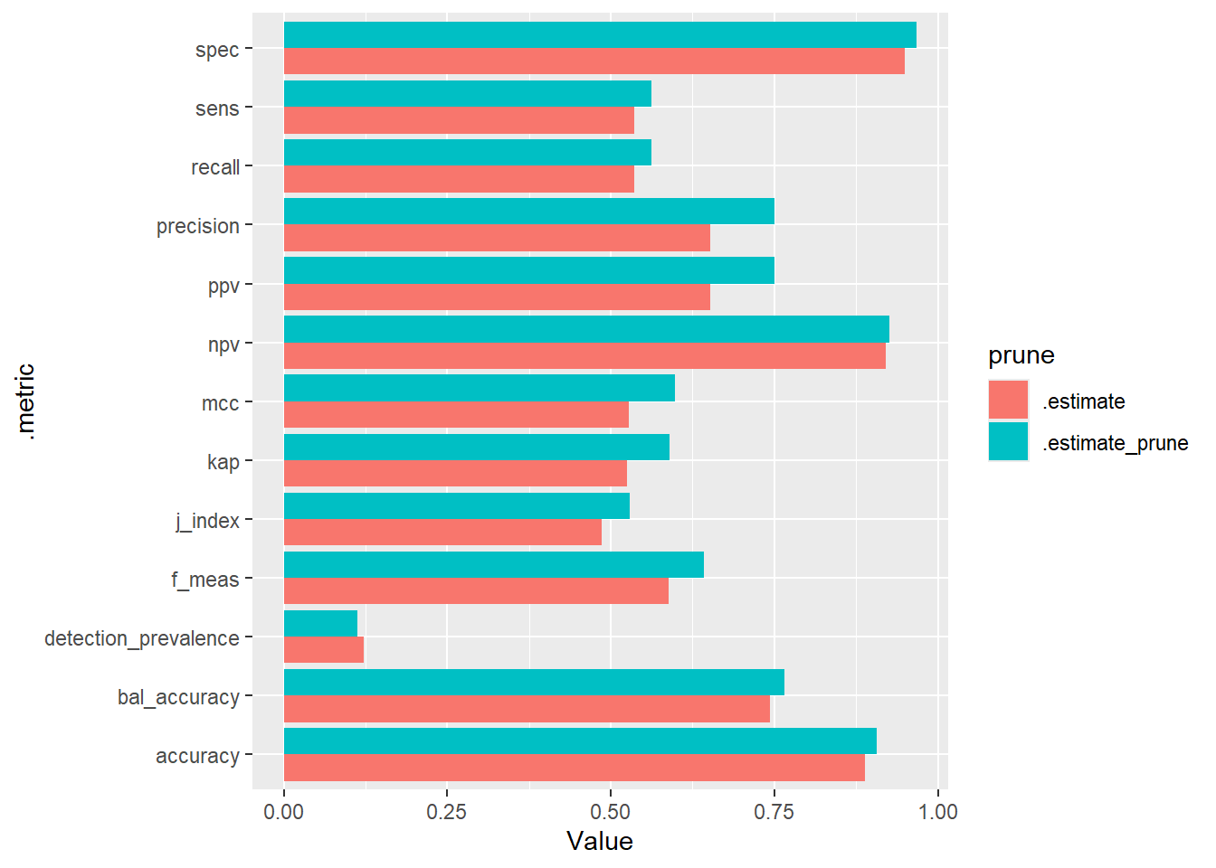

22.8 Compare ROC Curves

roc_auc.compare <- stacked_dfs %>%
  group_by(model_type) %>%
  roc_auc(truth=diq010, pred_prob)

roc_auc.compare

# A tibble: 2 × 4
  model_type .metric .estimator .estimate
  <chr>      <chr>   <chr>          <dbl>
1 not_pruned roc_auc binary         0.780
2 prune      roc_auc binary         0.765

roc_auc.compare2 <- roc_auc.compare %>%
  select(model_type, .estimate) %>% 
  spread(key='model_type',value='.estimate')

roc_auc.compare2

# A tibble: 1 × 2
  not_pruned prune
       <dbl> <dbl>
1      0.780 0.765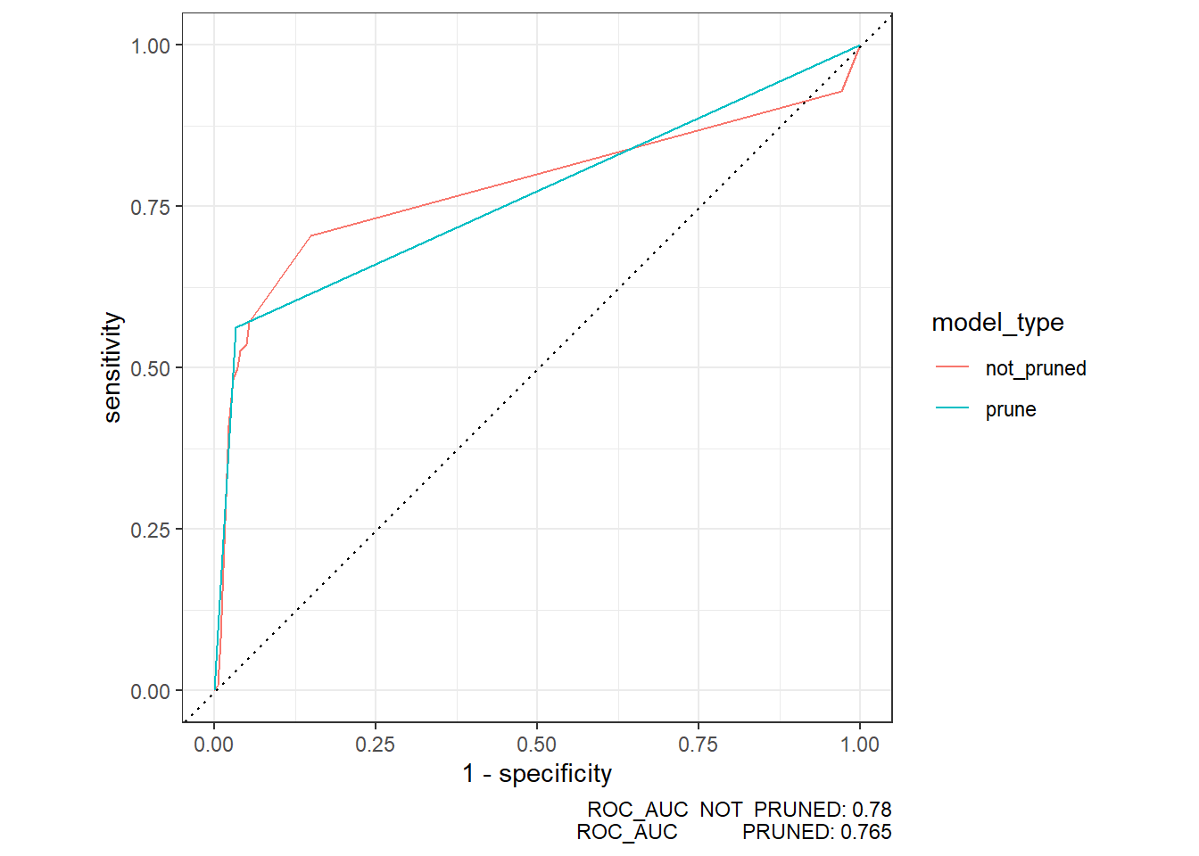

test_compare_roc <- stacked_dfs %>%
  group_by(model_type) %>%
  roc_curve(truth=diq010, pred_prob) 

autoplot(test_compare_roc) + 
 labs( caption = paste0("ROC_AUC  NOT  PRUNED: ", round(roc_auc.compare2$not_pruned,3) , 
                         "\nROC_AUC            PRUNED: ", round(roc_auc.compare2$prune,3) ) )

\(~\)

22.9 Compare Model Metrics - More Groups

diab_pop.test.stacked_dfs <- stacked_dfs %>% 
  left_join(diab_pop.no_na_vals.test, by = c("seqn", "diq010"))
  
rpart.plot(tree_1)

head(tree_1$splits,20)

         count ncat     improve  index        adj
lbxglu    1126    1 113.1344112 135.00 0.00000000
ridageyr  1126    1  22.8255083  48.50 0.00000000
bmxbmi    1126    1   7.6602898  27.65 0.00000000
dmdeduc2  1126    5   5.7790434   1.00 0.00000000
dmdmartl  1126    6   5.7449142   2.00 0.00000000
lbxglu     132    1   6.9602273 154.50 0.00000000
bmxbmi     132    1   4.1704107  25.25 0.00000000
indhhin2   132   14   2.8812328   3.00 0.00000000
ridageyr   132    1   2.3778555  27.50 0.00000000
dmdmartl   132    6   1.8782314   4.00 0.00000000
ridageyr     0    1   0.7424242  27.50 0.05555556
bmxbmi       0    1   0.7424242  20.85 0.05555556
indhhin2     0   14   0.7348485   5.00 0.02777778
indhhin2    96   14   1.7355769   6.00 0.00000000
bmxbmi      96   -1   1.0405963  37.20 0.00000000
ridreth1    96    5   0.5720238   7.00 0.00000000
dmdmartl    96    6   0.5628608   8.00 0.00000000
ridageyr    96    1   0.5208333  61.50 0.00000000
bmxbmi       0    1   0.8333333  21.35 0.11111111
lbxglu       0   -1   0.8333333 393.50 0.11111111

# let's use ridreth1

cm_compare_groups <- diab_pop.test.stacked_dfs %>%
  group_by(model_type,ridreth1) %>%
  conf_mat(truth = diq010, estimate = pred_class ) %>%
  ungroup()

cm_compare_groups

# A tibble: 10 × 3
   model_type ridreth1           conf_mat  
   <chr>      <fct>              <list>    
 1 not_pruned MexicanAmerican    <conf_mat>
 2 not_pruned Other Hispanic     <conf_mat>
 3 not_pruned Non-Hispanic White <conf_mat>
 4 not_pruned Non-Hispanic Black <conf_mat>
 5 not_pruned Other              <conf_mat>
 6 prune      MexicanAmerican    <conf_mat>
 7 prune      Other Hispanic     <conf_mat>
 8 prune      Non-Hispanic White <conf_mat>
 9 prune      Non-Hispanic Black <conf_mat>
10 prune      Other              <conf_mat>

str(cm_compare_groups,1)

tibble [10 × 3] (S3: tbl_df/tbl/data.frame)

cm_compare_groups[3,]$conf_mat[[1]]

             Truth
Prediction    Diabetes No Diabetes
  Diabetes          16          15
  No Diabetes       14         215

cm_compare_groups[3,c('model_type', 'ridreth1')]

# A tibble: 1 × 2
  model_type ridreth1          
  <chr>      <fct>             
1 not_pruned Non-Hispanic White

summary(cm_compare_groups$conf_mat[[3]])

# A tibble: 13 × 3
   .metric              .estimator .estimate
   <chr>                <chr>          <dbl>
 1 accuracy             binary         0.888
 2 kap                  binary         0.461
 3 sens                 binary         0.533
 4 spec                 binary         0.935
 5 ppv                  binary         0.516
 6 npv                  binary         0.939
 7 mcc                  binary         0.462
 8 j_index              binary         0.468
 9 bal_accuracy         binary         0.734
10 detection_prevalence binary         0.119
11 precision            binary         0.516
12 recall               binary         0.533
13 f_meas               binary         0.525

22.10 Compare Groups Helper Function

Group_Model_Metic_Compare_helper_fun <- function(my_data, my_row_number, ...) {
  
  group_var <- enquos(...)
  
  row_of_data <- my_data %>%
    filter(row_number() == my_row_number)

  summary_stats <- summary(row_of_data$conf_mat[[1]]) %>% 
    mutate(join_key = 1)
  
  row_of_data_2 <- row_of_data %>% 
    select(!!!  group_var) %>% 
    mutate(join_key = 1)
  
  output <- row_of_data_2 %>% 
    left_join(summary_stats, by = "join_key") %>%
    select(-join_key)
  
return(output)
}

22.10.1 Test Compare Groups Helper Function

Group_Model_Metic_Compare_helper_fun(cm_compare_groups, 3, model_type, ridreth1)

# A tibble: 13 × 5
   model_type ridreth1           .metric              .estimator .estimate
   <chr>      <fct>              <chr>                <chr>          <dbl>
 1 not_pruned Non-Hispanic White accuracy             binary         0.888
 2 not_pruned Non-Hispanic White kap                  binary         0.461
 3 not_pruned Non-Hispanic White sens                 binary         0.533
 4 not_pruned Non-Hispanic White spec                 binary         0.935
 5 not_pruned Non-Hispanic White ppv                  binary         0.516
 6 not_pruned Non-Hispanic White npv                  binary         0.939
 7 not_pruned Non-Hispanic White mcc                  binary         0.462
 8 not_pruned Non-Hispanic White j_index              binary         0.468
 9 not_pruned Non-Hispanic White bal_accuracy         binary         0.734
10 not_pruned Non-Hispanic White detection_prevalence binary         0.119
11 not_pruned Non-Hispanic White precision            binary         0.516
12 not_pruned Non-Hispanic White recall               binary         0.533
13 not_pruned Non-Hispanic White f_meas               binary         0.525

22.11 Apply Compare Groups Helper Function

list_to_apply_function <- 1:nrow(cm_compare_groups)

Final_Compare_Group_Table <- map_dfr(list_to_apply_function,
                                      Group_Model_Metic_Compare_helper_fun, 
                                      my_data = cm_compare_groups, 
                                      model_type, ridreth1)

Final_Compare_Group_Table

# A tibble: 130 × 5
   model_type ridreth1        .metric              .estimator .estimate
   <chr>      <fct>           <chr>                <chr>          <dbl>
 1 not_pruned MexicanAmerican accuracy             binary         0.832
 2 not_pruned MexicanAmerican kap                  binary         0.275
 3 not_pruned MexicanAmerican sens                 binary         0.286
 4 not_pruned MexicanAmerican spec                 binary         0.942
 5 not_pruned MexicanAmerican ppv                  binary         0.5  
 6 not_pruned MexicanAmerican npv                  binary         0.867
 7 not_pruned MexicanAmerican mcc                  binary         0.289
 8 not_pruned MexicanAmerican j_index              binary         0.228
 9 not_pruned MexicanAmerican bal_accuracy         binary         0.614
10 not_pruned MexicanAmerican detection_prevalence binary         0.096
# ℹ 120 more rows

22.11.1 Bar Graph of Model Metrics by Race/Hispanic Origin, Model Type, and Diabetes

ggplot(Final_Compare_Group_Table, aes(.metric, .estimate, fill = model_type)) + 
  geom_bar(stat="identity",  position=position_dodge()) +
  coord_flip() +
  facet_wrap(~ridreth1)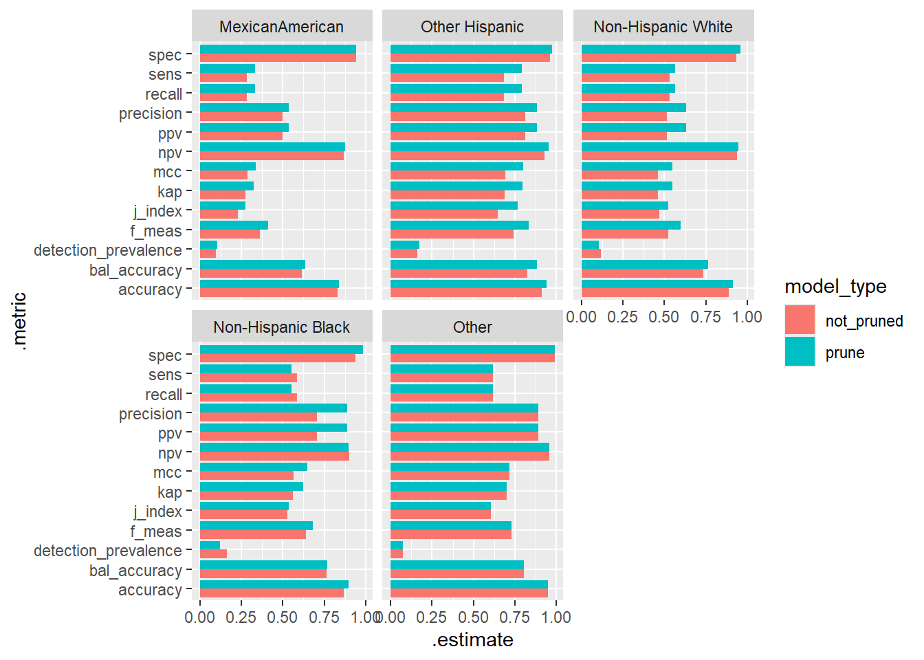

22.11.2 Multi-Group ROCs

Final_Compare_Group_Table.roc_auc <- diab_pop.test.stacked_dfs %>%
  group_by(model_type,ridreth1) %>% 
  roc_auc(truth=diq010, pred_prob)

ggplot(Final_Compare_Group_Table.roc_auc, aes(ridreth1, .estimate, fill = model_type)) + 
  geom_bar(stat="identity",  position=position_dodge()) +
  coord_flip()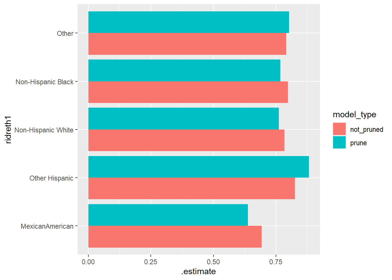

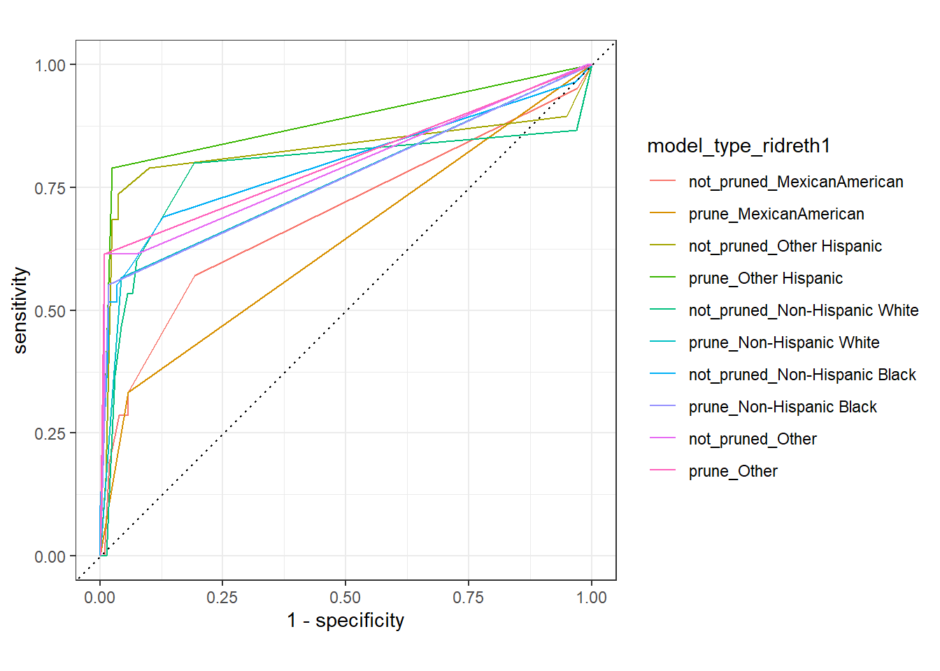
test_compare_groups_roc <- diab_pop.test.stacked_dfs %>%
  group_by(model_type,ridreth1) %>%
  roc_curve(truth=diq010, pred_prob) 

autoplot(test_compare_groups_roc)

autoplot(test_compare_groups_roc) +
  facet_wrap(~model_type)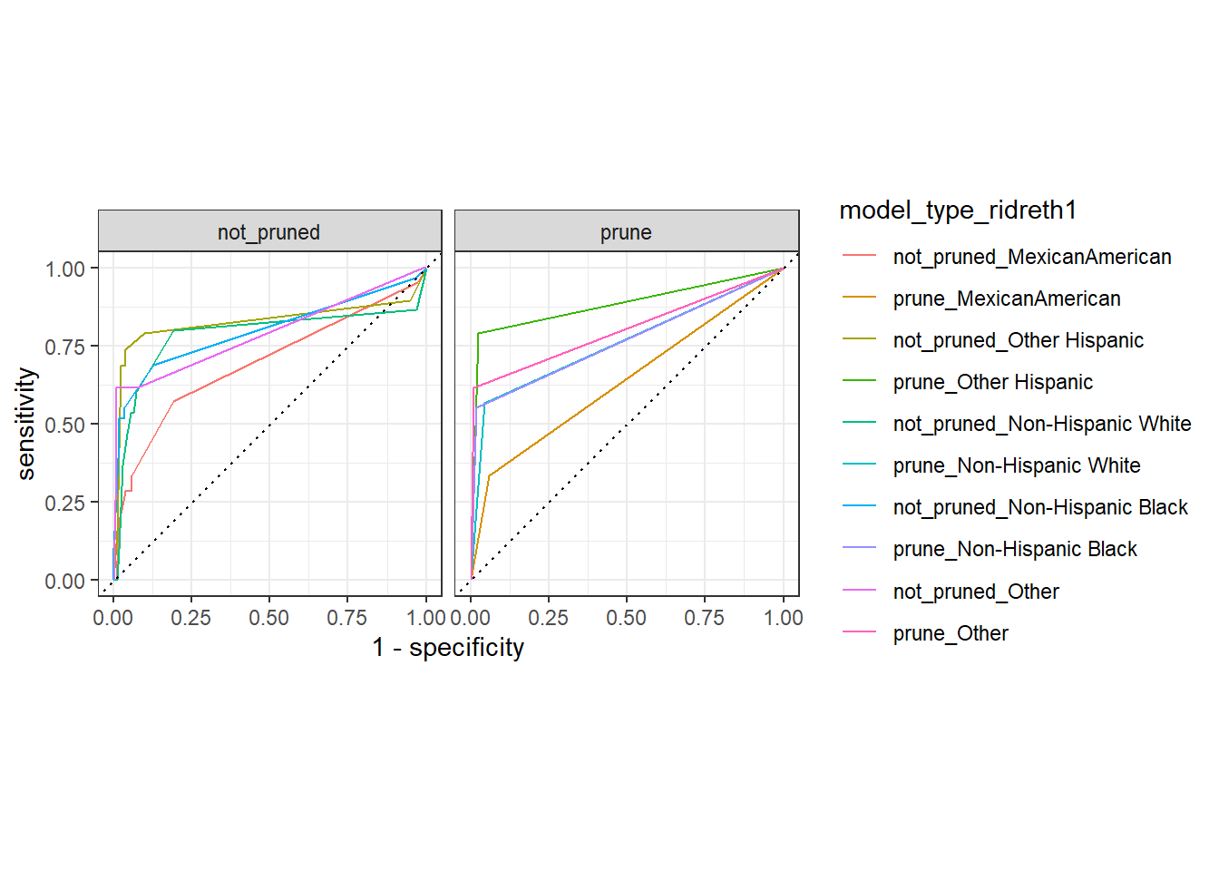

autoplot(test_compare_groups_roc) +
  facet_wrap(~ridreth1)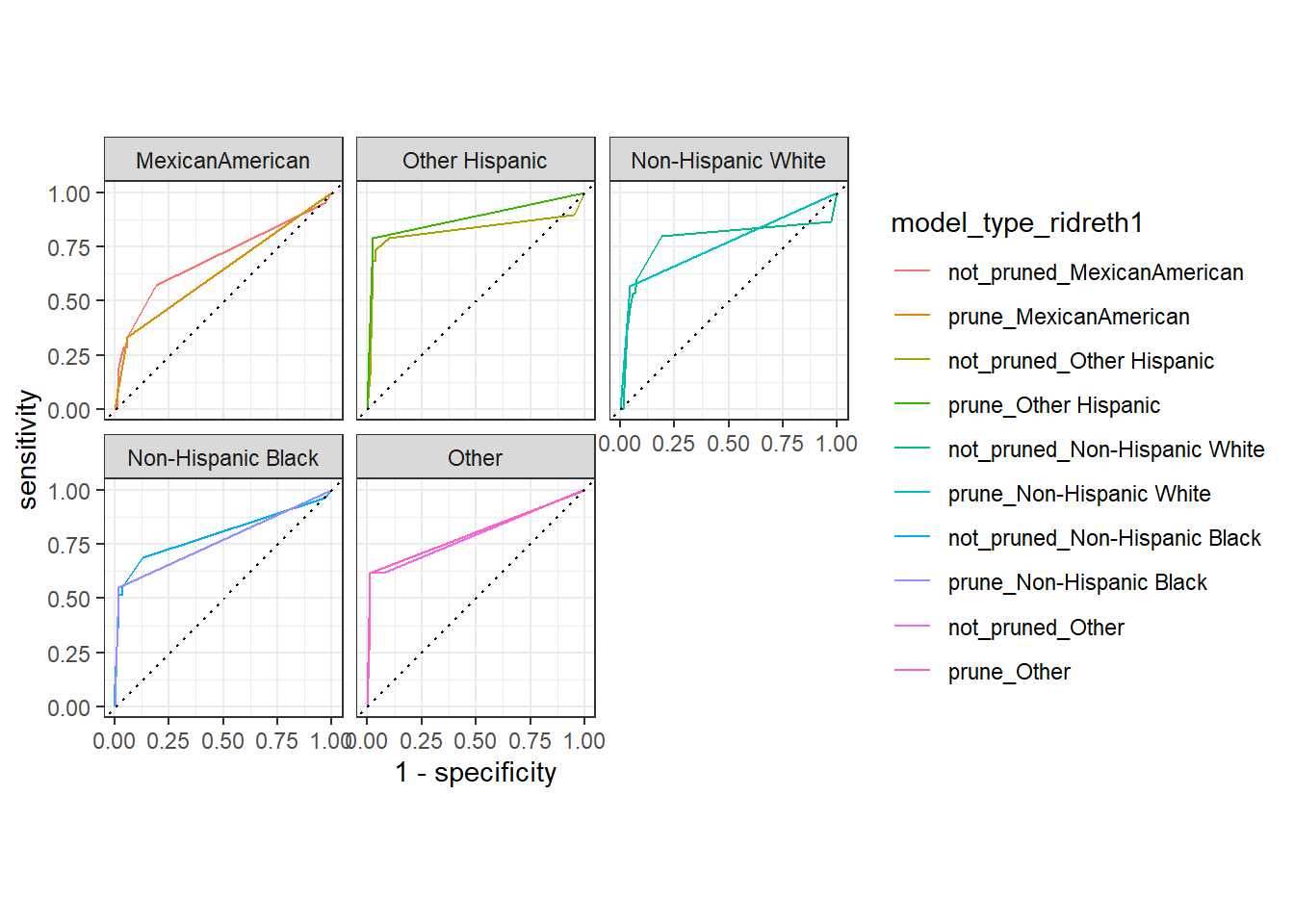

\(~\)

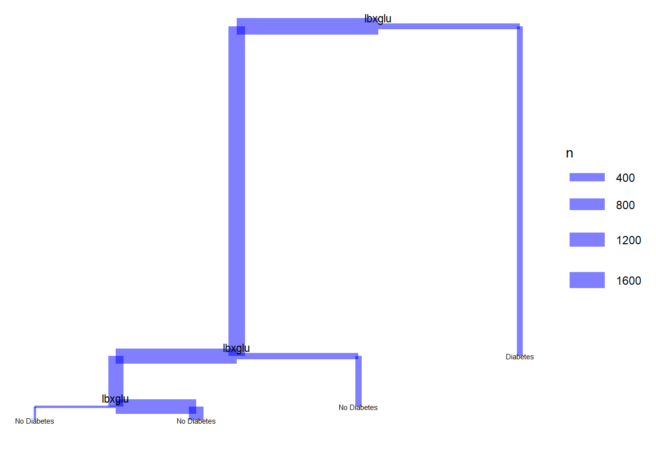
22.12 Dendrograms with `ggdendro`

\(~\)

library(ggplot2)
library(ggdendro)
library(tree)

  model <- tree(diq010 ~ riagendr + ridreth1 + indhhin2 + dmdeduc2 + dmdmartl + bmxbmi + lbxglu, 
                data = diab_pop)
  
  tree_data <- dendro_data(model)
  
  segment(tree_data) %>%
  ggplot() +
    geom_segment(aes(x = x, 
                     y = y, 
                     xend = xend, 
                     yend = yend, 
                     size = n), 
                 colour = "blue", alpha = 0.5) +
    scale_size("n") +
    geom_text(data = label(tree_data), 
              aes(x = x, y = y, label = label), vjust = -0.5, size = 3) +
    geom_text(data = leaf_label(tree_data), 
              aes(x = x, y = y, label = label), vjust = 0.5, size = 2) +
    theme_dendro()

Warning: Using `size` aesthetic for lines was deprecated in ggplot2 3.4.0.
ℹ Please use `linewidth` instead.

21.1 Reminders

21.1.1 Install if not Function

21.2 Data Prep

21.2.1 EDA and Imputation

21.3 Split Data with caret

21.3.1 Define the Training Set

21.3.2 Define the Testing Set

21.4 Fit Decision Trees with rpart

21.5 Better View with rpart.plot

21.6 rpart output

21.7 Prune Decision Tree

21.8 Score Decision Tree Model on Training Set

21.8.1 Score Output Probabilities

21.8.2 Score Output Class

21.8.3 View Training Dataset with Scores

21.9 Why was 135 chosen as the split value of lbxglu

21.9.1 Compare Confusion Matrix and 2-by-2 Tables

21.9.2 Programming a Confusion Matrix from a 2-by-2 Table

21.9.2.1 Check our work

21.10 Decision Tree - Choosing the Cut Point

21.10.1 Test lbxglu_value_chisq Function

21.11 Find Ranges

21.12 Apply Function

21.12.1 Sort Review Results

21.13 Plot Results

22 Score The Test Data

22.1 Use yardstick for Model Metrics

22.2 ROC Curve

22.3 Precision Recall Curve

22.4 Lift Curve

22.5 Gain Curve

22.6 Comparing Models

22.7 Compare Model Metrics

22.8 Compare ROC Curves

22.9 Compare Model Metrics - More Groups

22.10 Compare Groups Helper Function

22.10.1 Test Compare Groups Helper Function

22.11 Apply Compare Groups Helper Function

22.11.1 Bar Graph of Model Metrics by Race/Hispanic Origin, Model Type, and Diabetes

22.11.2 Multi-Group ROCs

22.12 Dendrograms with ggdendro

21.3 Split Data with `caret`

21.4 Fit Decision Trees with `rpart`

21.5 Better View with `rpart.plot`

21.6 `rpart` output

21.9 Why was 135 chosen as the split value of `lbxglu`

21.10.1 Test `lbxglu_value_chisq` Function

22.1 Use `yardstick` for Model Metrics

22.12 Dendrograms with `ggdendro`