10 Logistic Regression
10.1 Read in the Data
10.1.1 Reminders about the Data
tibble::tribble(
  ~"Variable in Data", ~"Definition", ~"Data Type",
  'seqn', 'Respondent sequence number', 'Identifier',
  'riagendr', 'Gender', 'Categorical',
  'ridageyr', 'Age in years at screening', 'Continuous / Numerical',
  'ridreth1', 'Race/Hispanic origin', 'Categorical',
  'dmdeduc2', 'Education level', 'Adults 20+  - Categorical',
  'dmdmartl', 'Marital status', 'Categorical',
  'indhhin2', 'Annual household income', 'Categorical',
  'bmxbmi', 'Body Mass Index (kg/m**2)', 'Continuous / Numerical',
  'diq010', 'Doctor diagnosed diabetes', 'Categorical',
  'lbxglu', 'Fasting Glucose (mg/dL)', 'Continuous / Numerical'
  ) |>
knitr::kable()| Variable in Data | Definition | Data Type |
|---|---|---|
| seqn | Respondent sequence number | Identifier |
| riagendr | Gender | Categorical |
| ridageyr | Age in years at screening | Continuous / Numerical |
| ridreth1 | Race/Hispanic origin | Categorical |
| dmdeduc2 | Education level | Adults 20+ - Categorical |
| dmdmartl | Marital status | Categorical |
| indhhin2 | Annual household income | Categorical |
| bmxbmi | Body Mass Index (kg/m**2) | Continuous / Numerical |
| diq010 | Doctor diagnosed diabetes | Categorical |
| lbxglu | Fasting Glucose (mg/dL) | Continuous / Numerical |
10.1.2 Install if not Function
install_if_not <- function( list.of.packages ) {
  new.packages <- list.of.packages[!(list.of.packages %in% installed.packages()[,"Package"])]
  if(length(new.packages)) { install.packages(new.packages) } else { print(paste0("the package '", list.of.packages , "' is already installed")) }
}
10.2 Split Data into Training and Test Sets.
── Attaching core tidyverse packages ──────────────────────── tidyverse 2.0.0 ──
✔ dplyr     1.2.1     ✔ readr     2.2.0
✔ forcats   1.0.1     ✔ stringr   1.6.0
✔ ggplot2   4.0.3     ✔ tibble    3.3.1
✔ lubridate 1.9.5     ✔ tidyr     1.3.2
✔ purrr     1.2.2
── Conflicts ────────────────────────────────────────── tidyverse_conflicts() ──
✖ dplyr::filter() masks stats::filter()
✖ dplyr::lag()    masks stats::lag()
ℹ Use the conflicted package (<http://conflicted.r-lib.org/>) to force all conflicts to become errorsLoading required package: lattice
Attaching package: 'caret'
The following object is masked from 'package:purrr':
liftthis will ensure our results are the same every run to randomize you may use: set.seed(Sys.time())
set.seed(8675309) The createDataPartition function is used to create training and test sets
trainIndex <- createDataPartition(diab_pop.no_na_vals$diq010,
                                  p = .6,
                                  list = FALSE,
                                  times = 1)
diab_pop.no_na_vals.train <- diab_pop.no_na_vals[trainIndex, ]
diab_pop.no_na_vals.test <- diab_pop.no_na_vals[-trainIndex, ]10.3 Train Logistic Regression Model
logit_model <- glm(diq010 ~ riagendr + ridageyr + ridreth1 + dmdeduc2 + dmdmartl + indhhin2 + bmxbmi + lbxglu,
                   family="binomial",
                   data = diab_pop.no_na_vals.train)

logit_model
Call:  glm(formula = diq010 ~ riagendr + ridageyr + ridreth1 + dmdeduc2 +
    dmdmartl + indhhin2 + bmxbmi + lbxglu, family = "binomial",
    data = diab_pop.no_na_vals.train)

Coefficients:
                       (Intercept)                      riagendrFemale
                           9.80789                            -0.11464
                          ridageyr              ridreth1Other Hispanic
                          -0.05503                            -0.29723
        ridreth1Non-Hispanic White          ridreth1Non-Hispanic Black
                          -0.38270                            -0.92228
                     ridreth1Other               dmdeduc2Grades 9-11th
                          -0.71991                             0.44575
  dmdeduc2High school graduate/GED  dmdeduc2Some college or AA degrees
                           1.26584                             0.90043
     dmdeduc2College grad or above                     dmdmartlWidowed
                           0.94730                             0.47483
                  dmdmartlDivorced                   dmdmartlSeparated
                           0.36843                            -0.04411
             dmdmartlNever married         dmdmartlLiving with partner
                          -0.03577                             0.17759
             indhhin2$5,000-$9,999             indhhin2$10,000-$14,999
                           0.34427                             1.52998
           indhhin2$15,000-$19,999             indhhin2$20,000-$24,999
                           1.78220                             1.08653
           indhhin2$25,000-$34,999             indhhin2$45,000-$54,999
                           1.04877                             0.75253
           indhhin2$65,000-$74,999                     indhhin220,000+
                           0.90369                             1.03068
         indhhin2less than $20,000             indhhin2$75,000-$99,999
                           2.72902                             1.41228
                 indhhin2$100,000+                              bmxbmi
                           0.77823                            -0.05353
                            lbxglu
                          -0.03826

Degrees of Freedom: 1125 Total (i.e. Null);  1097 Residual
Null Deviance:      952.3
Residual Deviance: 551.3 AIC: 609.3summary(logit_model)
Call:
glm(formula = diq010 ~ riagendr + ridageyr + ridreth1 + dmdeduc2 +
    dmdmartl + indhhin2 + bmxbmi + lbxglu, family = "binomial",
    data = diab_pop.no_na_vals.train)

Coefficients:
                                    Estimate Std. Error z value Pr(>|z|)
(Intercept)                         9.807888   1.143258   8.579  < 2e-16 ***
riagendrFemale                     -0.114638   0.238933  -0.480  0.63138
ridageyr                           -0.055027   0.009326  -5.900 3.63e-09 ***
ridreth1Other Hispanic             -0.297226   0.428658  -0.693  0.48807
ridreth1Non-Hispanic White         -0.382705   0.393014  -0.974  0.33017
ridreth1Non-Hispanic Black         -0.922281   0.418804  -2.202  0.02765 *
ridreth1Other                      -0.719906   0.487388  -1.477  0.13966
dmdeduc2Grades 9-11th               0.445749   0.429922   1.037  0.29982
dmdeduc2High school graduate/GED    1.265841   0.400733   3.159  0.00158 **
dmdeduc2Some college or AA degrees  0.900433   0.389046   2.314  0.02064 *
dmdeduc2College grad or above       0.947302   0.426745   2.220  0.02643 *
dmdmartlWidowed                     0.474834   0.399959   1.187  0.23515
dmdmartlDivorced                    0.368433   0.378205   0.974  0.32998
dmdmartlSeparated                  -0.044107   0.558009  -0.079  0.93700
dmdmartlNever married              -0.035769   0.437124  -0.082  0.93478
dmdmartlLiving with partner         0.177591   0.547438   0.324  0.74563
indhhin2$5,000-$9,999               0.344274   0.627713   0.548  0.58338
indhhin2$10,000-$14,999             1.529979   0.657454   2.327  0.01996 *
indhhin2$15,000-$19,999             1.782201   0.672002   2.652  0.00800 **
indhhin2$20,000-$24,999             1.086530   0.639608   1.699  0.08937 .
indhhin2$25,000-$34,999             1.048766   0.590010   1.778  0.07548 .
indhhin2$45,000-$54,999             0.752527   0.632012   1.191  0.23378
indhhin2$65,000-$74,999             0.903686   0.656972   1.376  0.16897
indhhin220,000+                     1.030682   0.902598   1.142  0.25349
indhhin2less than $20,000           2.729024   1.140925   2.392  0.01676 *
indhhin2$75,000-$99,999             1.412279   0.657736   2.147  0.03178 *
indhhin2$100,000+                   0.778230   0.615139   1.265  0.20582
bmxbmi                             -0.053526   0.017057  -3.138  0.00170 **
lbxglu                             -0.038258   0.003688 -10.373  < 2e-16 ***
---
Signif. codes:  0 '***' 0.001 '**' 0.01 '*' 0.05 '.' 0.1 ' ' 1

(Dispersion parameter for binomial family taken to be 1)

    Null deviance: 952.29  on 1125  degrees of freedom
Residual deviance: 551.29  on 1097  degrees of freedom
AIC: 609.29

Number of Fisher Scoring iterations: 6str(logit_model,1)List of 30
$ coefficients : Named num [1:29] 9.808 -0.115 -0.055 -0.297 -0.383 ...
..- attr(*, "names")= chr [1:29] "(Intercept)" "riagendrFemale" "ridageyr" "ridreth1Other Hispanic" ...
$ residuals : Named num [1:1126] 1.01 1.03 1.68 -1.01 1.13 ...
..- attr(*, "names")= chr [1:1126] "2" "11" "13" "14" ...
$ fitted.values : Named num [1:1126] 0.98802 0.96838 0.59693 0.00902 0.88719 ...
..- attr(*, "names")= chr [1:1126] "2" "11" "13" "14" ...
$ effects : Named num [1:1126] -12.493 0.103 6.2 -0.463 2.082 ...
..- attr(*, "names")= chr [1:1126] "(Intercept)" "riagendrFemale" "ridageyr" "ridreth1Other Hispanic" ...
$ R : num [1:29, 1:29] -8.93 0 0 0 0 ...
..- attr(*, "dimnames")=List of 2
$ rank : int 29
$ qr :List of 5
..- attr(*, "class")= chr "qr"
$ family :List of 13
..- attr(*, "class")= chr "family"
$ linear.predictors: Named num [1:1126] 4.413 3.422 0.393 -4.699 2.062 ...
..- attr(*, "names")= chr [1:1126] "2" "11" "13" "14" ...
$ deviance : num 551
$ aic : num 609
$ null.deviance : num 952
$ iter : int 6
$ weights : Named num [1:1126] 0.01184 0.03062 0.2406 0.00894 0.10009 ...
..- attr(*, "names")= chr [1:1126] "2" "11" "13" "14" ...
$ prior.weights : Named num [1:1126] 1 1 1 1 1 1 1 1 1 1 ...
..- attr(*, "names")= chr [1:1126] "2" "11" "13" "14" ...
$ df.residual : int 1097
$ df.null : int 1125
$ y : Named num [1:1126] 1 1 1 0 1 1 1 1 1 1 ...
..- attr(*, "names")= chr [1:1126] "2" "11" "13" "14" ...
$ converged : logi TRUE
$ boundary : logi FALSE
$ model :'data.frame': 1126 obs. of 9 variables:
..- attr(*, "terms")=Classes 'terms', 'formula' language diq010 ~ riagendr + ridageyr + ridreth1 + dmdeduc2 + dmdmartl + indhhin2 + bmxbmi + lbxglu
.. .. ..- attr(*, "variables")= language list(diq010, riagendr, ridageyr, ridreth1, dmdeduc2, dmdmartl, indhhin2, bmxbmi, lbxglu)
.. .. ..- attr(*, "factors")= int [1:9, 1:8] 0 1 0 0 0 0 0 0 0 0 ...
.. .. .. ..- attr(*, "dimnames")=List of 2
.. .. ..- attr(*, "term.labels")= chr [1:8] "riagendr" "ridageyr" "ridreth1" "dmdeduc2" ...
.. .. ..- attr(*, "order")= int [1:8] 1 1 1 1 1 1 1 1
.. .. ..- attr(*, "intercept")= int 1
.. .. ..- attr(*, "response")= int 1
.. .. ..- attr(*, ".Environment")=<environment: R_GlobalEnv>
.. .. ..- attr(*, "predvars")= language list(diq010, riagendr, ridageyr, ridreth1, dmdeduc2, dmdmartl, indhhin2, bmxbmi, lbxglu)
.. .. ..- attr(*, "dataClasses")= Named chr [1:9] "factor" "factor" "numeric" "factor" ...
.. .. .. ..- attr(*, "names")= chr [1:9] "diq010" "riagendr" "ridageyr" "ridreth1" ...
$ call : language glm(formula = diq010 ~ riagendr + ridageyr + ridreth1 + dmdeduc2 + dmdmartl + indhhin2 + bmxbmi + lbxglu, fa| __truncated__
$ formula :Class 'formula' language diq010 ~ riagendr + ridageyr + ridreth1 + dmdeduc2 + dmdmartl + indhhin2 + bmxbmi + lbxglu
.. ..- attr(*, ".Environment")=<environment: R_GlobalEnv>
$ terms :Classes 'terms', 'formula' language diq010 ~ riagendr + ridageyr + ridreth1 + dmdeduc2 + dmdmartl + indhhin2 + bmxbmi + lbxglu
.. ..- attr(*, "variables")= language list(diq010, riagendr, ridageyr, ridreth1, dmdeduc2, dmdmartl, indhhin2, bmxbmi, lbxglu)
.. ..- attr(*, "factors")= int [1:9, 1:8] 0 1 0 0 0 0 0 0 0 0 ...
.. .. ..- attr(*, "dimnames")=List of 2
.. ..- attr(*, "term.labels")= chr [1:8] "riagendr" "ridageyr" "ridreth1" "dmdeduc2" ...
.. ..- attr(*, "order")= int [1:8] 1 1 1 1 1 1 1 1
.. ..- attr(*, "intercept")= int 1
.. ..- attr(*, "response")= int 1
.. ..- attr(*, ".Environment")=<environment: R_GlobalEnv>
.. ..- attr(*, "predvars")= language list(diq010, riagendr, ridageyr, ridreth1, dmdeduc2, dmdmartl, indhhin2, bmxbmi, lbxglu)
.. ..- attr(*, "dataClasses")= Named chr [1:9] "factor" "factor" "numeric" "factor" ...
.. .. ..- attr(*, "names")= chr [1:9] "diq010" "riagendr" "ridageyr" "ridreth1" ...
$ data :'data.frame': 1126 obs. of 10 variables:
..- attr(*, "na.action")= 'omit' Named int [1:3843] 1 4 5 7 8 9 10 12 16 18 ...
.. ..- attr(*, "names")= chr [1:3843] "1" "4" "5" "7" ...
$ offset : NULL
$ control :List of 3
$ method : chr "glm.fit"
$ contrasts :List of 5
$ xlevels :List of 5
- attr(*, "class")= chr [1:2] "glm" "lm"logit_model$coefficients (Intercept) riagendrFemale
9.80788800 -0.11463826
ridageyr ridreth1Other Hispanic
-0.05502652 -0.29722567
ridreth1Non-Hispanic White ridreth1Non-Hispanic Black
-0.38270466 -0.92228099
ridreth1Other dmdeduc2Grades 9-11th
-0.71990619 0.44574943
dmdeduc2High school graduate/GED dmdeduc2Some college or AA degrees
1.26584123 0.90043329
dmdeduc2College grad or above dmdmartlWidowed
0.94730185 0.47483393
dmdmartlDivorced dmdmartlSeparated
0.36843309 -0.04410658
dmdmartlNever married dmdmartlLiving with partner
-0.03576914 0.17759058
indhhin2$5,000-$9,999 indhhin2$10,000-$14,999
0.34427417 1.52997906
indhhin2$15,000-$19,999 indhhin2$20,000-$24,999
1.78220109 1.08652981
indhhin2$25,000-$34,999 indhhin2$45,000-$54,999
1.04876567 0.75252721
indhhin2$65,000-$74,999 indhhin220,000+
0.90368602 1.03068174
indhhin2less than $20,000 indhhin2$75,000-$99,999
2.72902414 1.41227935
indhhin2$100,000+ bmxbmi
0.77823046 -0.05352607
lbxglu
-0.03825800 logit_model$aic[1] 609.2867coeff_logit_model <- broom::tidy(logit_model)
coeff_logit_model# A tibble: 29 × 5
term estimate std.error statistic p.value
<chr> <dbl> <dbl> <dbl> <dbl>
1 (Intercept) 9.81 1.14 8.58 9.58e-18
2 riagendrFemale -0.115 0.239 -0.480 6.31e- 1
3 ridageyr -0.0550 0.00933 -5.90 3.63e- 9
4 ridreth1Other Hispanic -0.297 0.429 -0.693 4.88e- 1
5 ridreth1Non-Hispanic White -0.383 0.393 -0.974 3.30e- 1
6 ridreth1Non-Hispanic Black -0.922 0.419 -2.20 2.77e- 2
7 ridreth1Other -0.720 0.487 -1.48 1.40e- 1
8 dmdeduc2Grades 9-11th 0.446 0.430 1.04 3.00e- 1
9 dmdeduc2High school graduate/GED 1.27 0.401 3.16 1.58e- 3
10 dmdeduc2Some college or AA degrees 0.900 0.389 2.31 2.06e- 2
# ℹ 19 more rows# A tibble: 29 × 6
term estimate std.error statistic p.value odds_ratio
<chr> <dbl> <dbl> <dbl> <dbl> <dbl>
1 (Intercept) 9.81 1.14 8.58 9.58e-18 18177.
2 indhhin2less than $20,000 2.73 1.14 2.39 1.68e- 2 15.3
3 indhhin2$15,000-$19,999 1.78 0.672 2.65 8.00e- 3 5.94
4 indhhin2$10,000-$14,999 1.53 0.657 2.33 2.00e- 2 4.62
5 indhhin2$75,000-$99,999 1.41 0.658 2.15 3.18e- 2 4.11
6 dmdeduc2High school graduat… 1.27 0.401 3.16 1.58e- 3 3.55
7 indhhin2$20,000-$24,999 1.09 0.640 1.70 8.94e- 2 2.96
8 indhhin2$25,000-$34,999 1.05 0.590 1.78 7.55e- 2 2.85
9 indhhin220,000+ 1.03 0.903 1.14 2.53e- 1 2.80
10 dmdeduc2College grad or abo… 0.947 0.427 2.22 2.64e- 2 2.58
# ℹ 19 more rows10.4 Score Testing Data
Since training data was used to train the model, we use the hold-out data or testing data to evaluate the model performance:
probs <- predict(logit_model, diab_pop.no_na_vals.test, "response")Rows: 750
Columns: 11
$ seqn <dbl> 83734, 83737, 83757, 83761, 83789, 83820, 83822, 83823, 83834…
$ riagendr <fct> Male, Female, Female, Female, Male, Male, Female, Female, Mal…
$ ridageyr <dbl> 78, 72, 57, 24, 66, 70, 20, 29, 69, 71, 37, 49, 41, 54, 80, 3…
$ ridreth1 <fct> Non-Hispanic White, MexicanAmerican, Other Hispanic, Other, N…
$ dmdeduc2 <fct> High school graduate/GED, Grades 9-11th, Less than 9th grade,…
$ dmdmartl <fct> Married, Separated, Separated, Never married, Living with par…
$ indhhin2 <fct> "$20,000-$24,999", "$75,000-$99,999", "$20,000-$24,999", "$0-…
$ bmxbmi <dbl> 28.8, 28.6, 35.4, 25.3, 34.0, 27.0, 22.2, 29.7, 28.2, 27.6, 3…
$ diq010 <fct> Diabetes, No Diabetes, Diabetes, No Diabetes, No Diabetes, No…
$ lbxglu <dbl> 84, 107, 398, 95, 113, 94, 80, 102, 105, 76, 79, 126, 110, 99…
$ probs <dbl> 9.387889e-01, 8.722288e-01, 5.437387e-05, 9.727618e-01, 8.427…
10.5 Use yardstick for Model Metrics
install_if_not('yardstick')[1] "the package 'yardstick' is already installed"
Attaching package: 'yardstick'The following objects are masked from 'package:caret':
precision, recall, sensitivity, specificityThe following object is masked from 'package:readr':
spec10.6 Confusion Matrix
A Confusion Matrix is a table of counts of classses for predicted classes versus actual classes. Therefore, in order to create a confusion matrix we will need to specify a threshold value for the probability; let’s use .5 and the conf_mat function:
Rows: 750
Columns: 12
$ seqn     <dbl> 83734, 83737, 83757, 83761, 83789, 83820, 83822, 83823, 83834…
$ riagendr <fct> Male, Female, Female, Female, Male, Male, Female, Female, Mal…
$ ridageyr <dbl> 78, 72, 57, 24, 66, 70, 20, 29, 69, 71, 37, 49, 41, 54, 80, 3…
$ ridreth1 <fct> Non-Hispanic White, MexicanAmerican, Other Hispanic, Other, N…
$ dmdeduc2 <fct> High school graduate/GED, Grades 9-11th, Less than 9th grade,…
$ dmdmartl <fct> Married, Separated, Separated, Never married, Living with par…
$ indhhin2 <fct> "$20,000-$24,999", "$75,000-$99,999", "$20,000-$24,999", "$0-…
$ bmxbmi   <dbl> 28.8, 28.6, 35.4, 25.3, 34.0, 27.0, 22.2, 29.7, 28.2, 27.6, 3…
$ diq010   <fct> Diabetes, No Diabetes, Diabetes, No Diabetes, No Diabetes, No…
$ lbxglu   <dbl> 84, 107, 398, 95, 113, 94, 80, 102, 105, 76, 79, 126, 110, 99…
$ probs    <dbl> 9.387889e-01, 8.722288e-01, 5.437387e-05, 9.727618e-01, 8.427…
$ Pred_DM2 <fct> No Diabetes, No Diabetes, Diabetes, No Diabetes, No Diabetes,… Truth
Prediction Diabetes No Diabetes
Diabetes 47 12
No Diabetes 65 626summary(conf_mat.logit)# A tibble: 13 × 3
.metric .estimator .estimate
<chr> <chr> <dbl>
1 accuracy binary 0.897
2 kap binary 0.498
3 sens binary 0.420
4 spec binary 0.981
5 ppv binary 0.797
6 npv binary 0.906
7 mcc binary 0.531
8 j_index binary 0.401
9 bal_accuracy binary 0.700
10 detection_prevalence binary 0.0787
11 precision binary 0.797
12 recall binary 0.420
13 f_meas binary 0.550 10.7 Receiver Operating Characteristic (ROC) Curve
The Receiver Operating Characteristic Curve or ROC Curve is created by plotting the true positive rate (TPR) against the false positive rate (FPR) at various threshold settings. The function roc_auc can be used to obtain the estimated area under the ROC curve and the function roc_curve can be used to plot the curve:
# A tibble: 1 × 3
  .metric .estimator .estimate
  <chr>   <chr>          <dbl>
1 roc_auc binary         0.854
diab_pop.no_na_vals.test.SCORED %>%
roc_curve(truth=diq010 , probs, event_level = 'second') %>%
autoplot() +
labs( title = "ROC Curve - Logistic Regression",
caption = paste0("Area Under ROC Curve : ",
round(roc_auc.logit$.estimate,3) ) ) +
theme( plot.title = element_text(size = 18) ,
plot.caption = element_text(size = 12))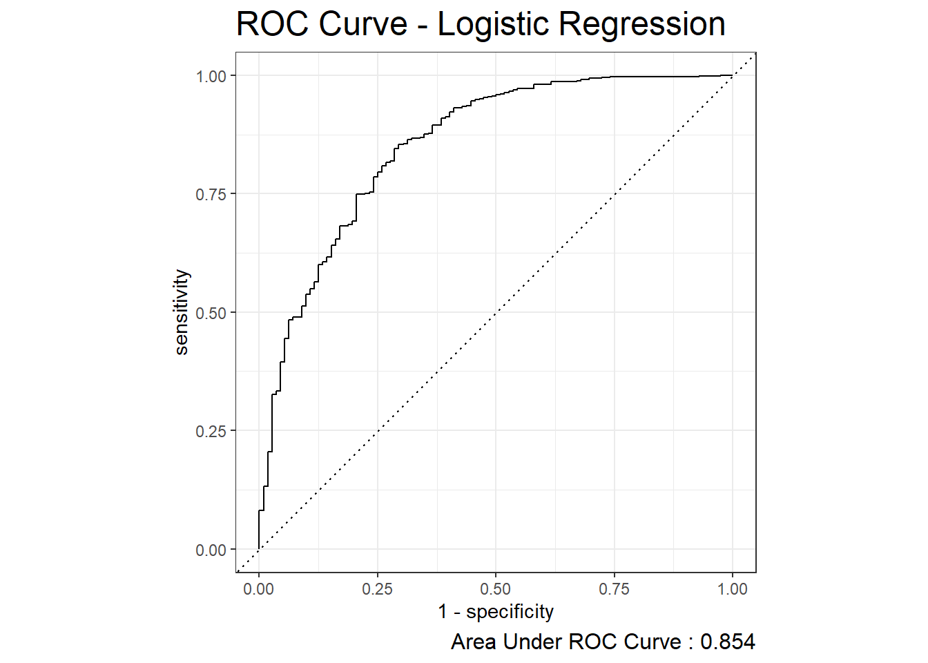
diab_pop.no_na_vals.test.SCORED %>%
  roc_curve(truth=diq010 , probs, event_level = 'second') %>%
  mutate(one_minus_spec = 1- specificity ) %>%
  ggplot(aes(x=one_minus_spec, y = sensitivity)) +
  geom_point() +
  labs( title = "ROC Curve - Logistic Regression",
        caption = paste0("Area Under ROC Curve : ",
                         round(roc_auc.logit$.estimate,3) )  ) +
  theme( plot.title = element_text(size = 18) ,
         plot.caption = element_text(size = 12))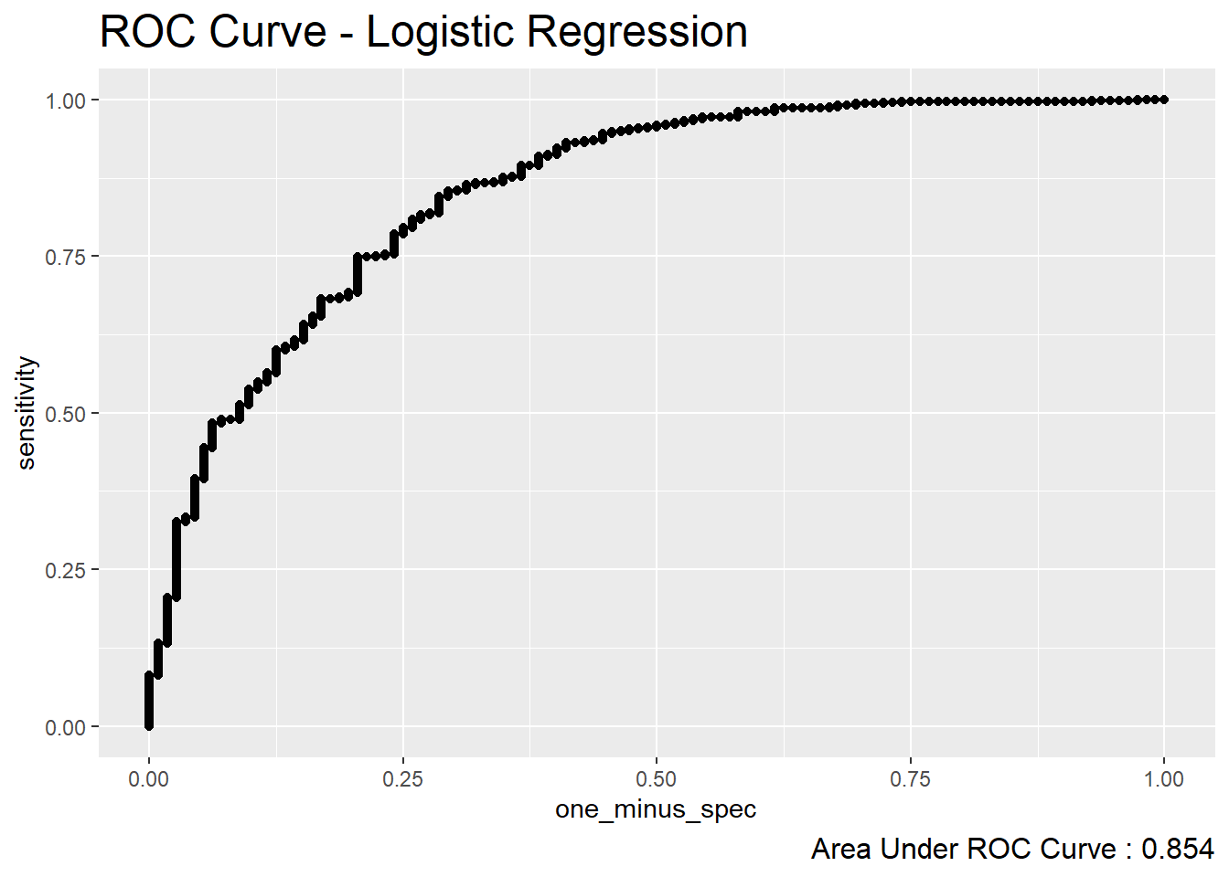
10.8 Precision-Recall Curve
The Precision-Recall Curve is created by plotting the precision or PPV against the recall or TPR at various threshold settings. The function pr_auc can be used to obtain the estimated area under the Precision-Recall Curve and the function pr_curve can be used to plot the curve:
# A tibble: 1 × 3
  .metric .estimator .estimate
  <chr>   <chr>          <dbl>
1 pr_auc  binary         0.965
diab_pop.no_na_vals.test.SCORED %>%
pr_curve(truth=diq010 , probs, event_level = 'second') %>%
autoplot() +
labs( title = "Precision-Recall Curve - Logistic Regression",
caption = paste0("Area Under Precision-Recall Curve : ", round(pr_auc.logit$.estimate,3) ) ) +
theme( plot.title = element_text(size = 18) ,
plot.caption = element_text(size = 12))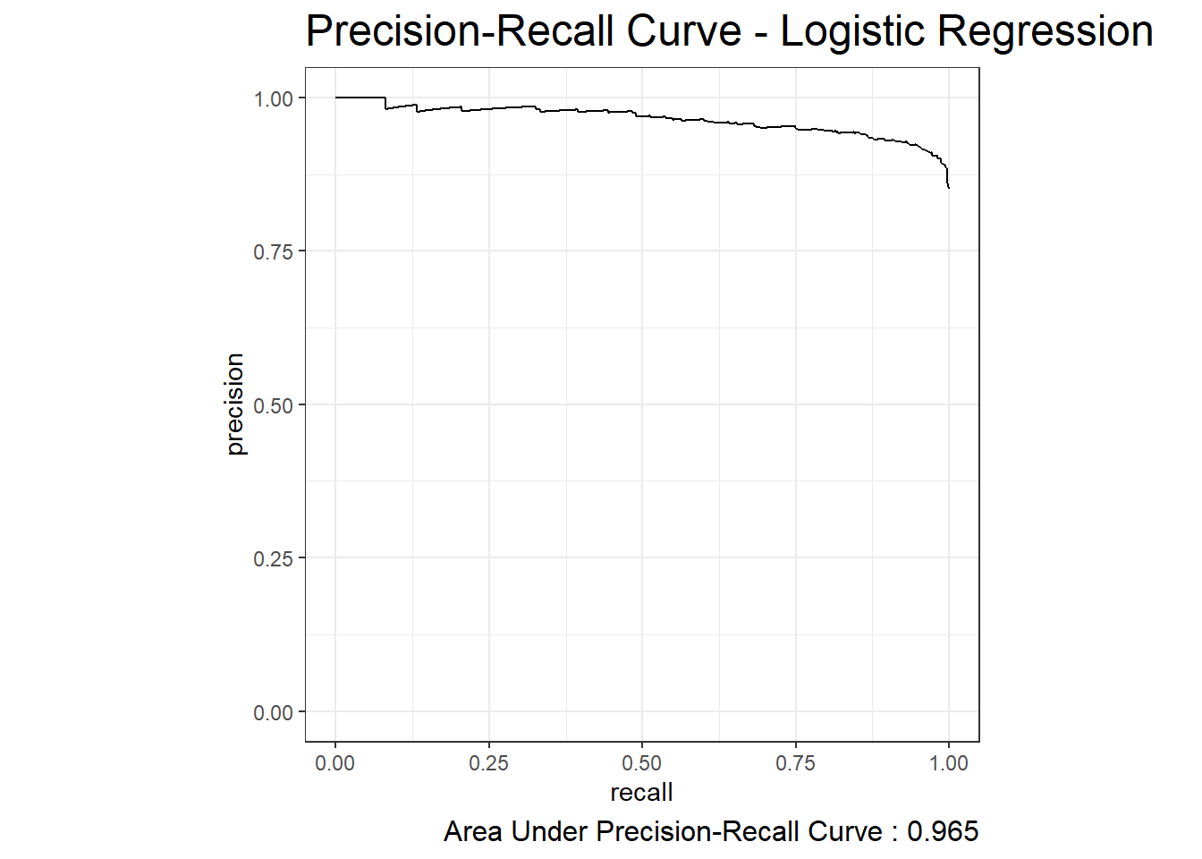
10.9 Lift Curve
lift_curve.logit <- diab_pop.no_na_vals.test.SCORED %>%
  lift_curve(truth=diq010, probs, event_level = 'second')

autoplot(lift_curve.logit) +
  labs( title = "Lift Curve - Logistic Regression") +
  theme(plot.title = element_text(size = 18))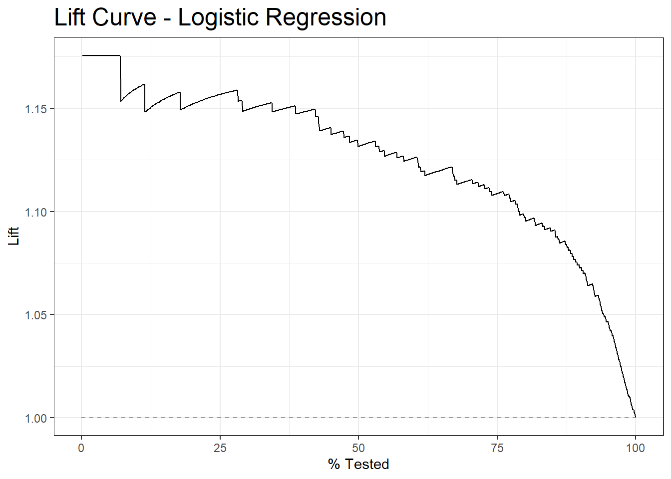
10.10 Gain Curve
gain_curve.logit <- diab_pop.no_na_vals.test.SCORED %>%
  gain_curve(truth=diq010, probs, event_level = 'second')

plot_gain_curve.logit <- autoplot(gain_curve.logit) +
  labs( title = "Gain Curve - Logistic Regression") +
  theme(plot.title = element_text(size = 18))

plot_gain_curve.logit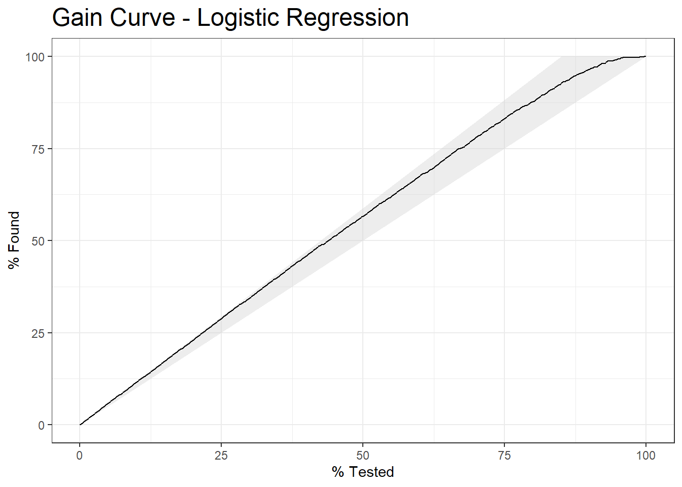
11 Train Logistic Regression Model No Intercept
Let’s remove the intercept and the variable lbxglu :
[1] "diq010 ~ riagendr + ridageyr + ridreth1 + dmdeduc2 + dmdmartl + indhhin2 + bmxbmi - 1"logit_no_int_model <- glm(formula_2,
family="binomial",
data = diab_pop.no_na_vals.train)
logit_no_int_model
Call:  glm(formula = formula_2, family = "binomial", data = diab_pop.no_na_vals.train)

Coefficients:
                      riagendrMale                      riagendrFemale
                           5.48435                             5.55488
                          ridageyr              ridreth1Other Hispanic
                          -0.05793                            -0.10096
        ridreth1Non-Hispanic White          ridreth1Non-Hispanic Black
                           0.23968                            -0.50310
                     ridreth1Other               dmdeduc2Grades 9-11th
                          -0.18278                             0.52285
  dmdeduc2High school graduate/GED  dmdeduc2Some college or AA degrees
                           0.84767                             0.82258
     dmdeduc2College grad or above                     dmdmartlWidowed
                           0.70671                             0.50172
                  dmdmartlDivorced                   dmdmartlSeparated
                           0.07506                            -0.10449
             dmdmartlNever married         dmdmartlLiving with partner
                           0.35830                             0.14843
             indhhin2$5,000-$9,999             indhhin2$10,000-$14,999
                           0.23534                             1.07971
           indhhin2$15,000-$19,999             indhhin2$20,000-$24,999
                           0.81281                             0.39890
           indhhin2$25,000-$34,999             indhhin2$45,000-$54,999
                           0.51096                             0.18778
           indhhin2$65,000-$74,999                     indhhin220,000+
                           0.99847                             0.51638
         indhhin2less than $20,000             indhhin2$75,000-$99,999
                           1.40105                             0.78987
                 indhhin2$100,000+                              bmxbmi
                           0.64519                            -0.06104

Degrees of Freedom: 1126 Total (i.e. Null);  1098 Residual
Null Deviance:      1561
Residual Deviance: 796.5    AIC: 852.5
11.1 Compare Models
Finally, we will compare the two models. First, score the test data with the model:
probs_no_int <- predict(logit_no_int_model, diab_pop.no_na_vals.test, "response")Now we combine with our previous results and use a gather to stack the results into the column value:
diab_pop.no_na_vals.test.SCORED_Compare <- cbind(diab_pop.no_na_vals.test.SCORED, probs_no_int)

diab_pop.no_na_vals.test.SCORED_Compare <- diab_pop.no_na_vals.test.SCORED_Compare %>%
  tidyr::gather(probs, probs_no_int, key="model_type", value = "value")

glimpse(diab_pop.no_na_vals.test.SCORED_Compare)
Rows: 1,500
Columns: 13
$ seqn <dbl> 83734, 83737, 83757, 83761, 83789, 83820, 83822, 83823, 838…
$ riagendr <fct> Male, Female, Female, Female, Male, Male, Female, Female, M…
$ ridageyr <dbl> 78, 72, 57, 24, 66, 70, 20, 29, 69, 71, 37, 49, 41, 54, 80,…
$ ridreth1 <fct> Non-Hispanic White, MexicanAmerican, Other Hispanic, Other,…
$ dmdeduc2 <fct> High school graduate/GED, Grades 9-11th, Less than 9th grad…
$ dmdmartl <fct> Married, Separated, Separated, Never married, Living with p…
$ indhhin2 <fct> "$20,000-$24,999", "$75,000-$99,999", "$20,000-$24,999", "$…
$ bmxbmi <dbl> 28.8, 28.6, 35.4, 25.3, 34.0, 27.0, 22.2, 29.7, 28.2, 27.6,…
$ diq010 <fct> Diabetes, No Diabetes, Diabetes, No Diabetes, No Diabetes, …
$ lbxglu <dbl> 84, 107, 398, 95, 113, 94, 80, 102, 105, 76, 79, 126, 110, …
$ Pred_DM2 <fct> No Diabetes, No Diabetes, Diabetes, No Diabetes, No Diabete…
$ model_type <chr> "probs", "probs", "probs", "probs", "probs", "probs", "prob…
$ value <dbl> 9.387889e-01, 8.722288e-01, 5.437387e-05, 9.727618e-01, 8.4…Now we can use roc_auc and roc_curve with a group_by on the key we added in the last step:
# A tibble: 2 × 4
  model_type   .metric .estimator .estimate
  <chr>        <chr>   <chr>          <dbl>
1 probs        roc_auc binary         0.854
2 probs_no_int roc_auc binary         0.753
diab_pop.no_na_vals.test.SCORED_Compare %>%
group_by(model_type) %>%
roc_curve(truth=diq010 , value, event_level = 'second') %>%
autoplot() +
labs( title = "ROC Curves - Logistic Regression Compare ") +
theme( plot.title = element_text(size = 18) ,
plot.caption = element_text(size = 12))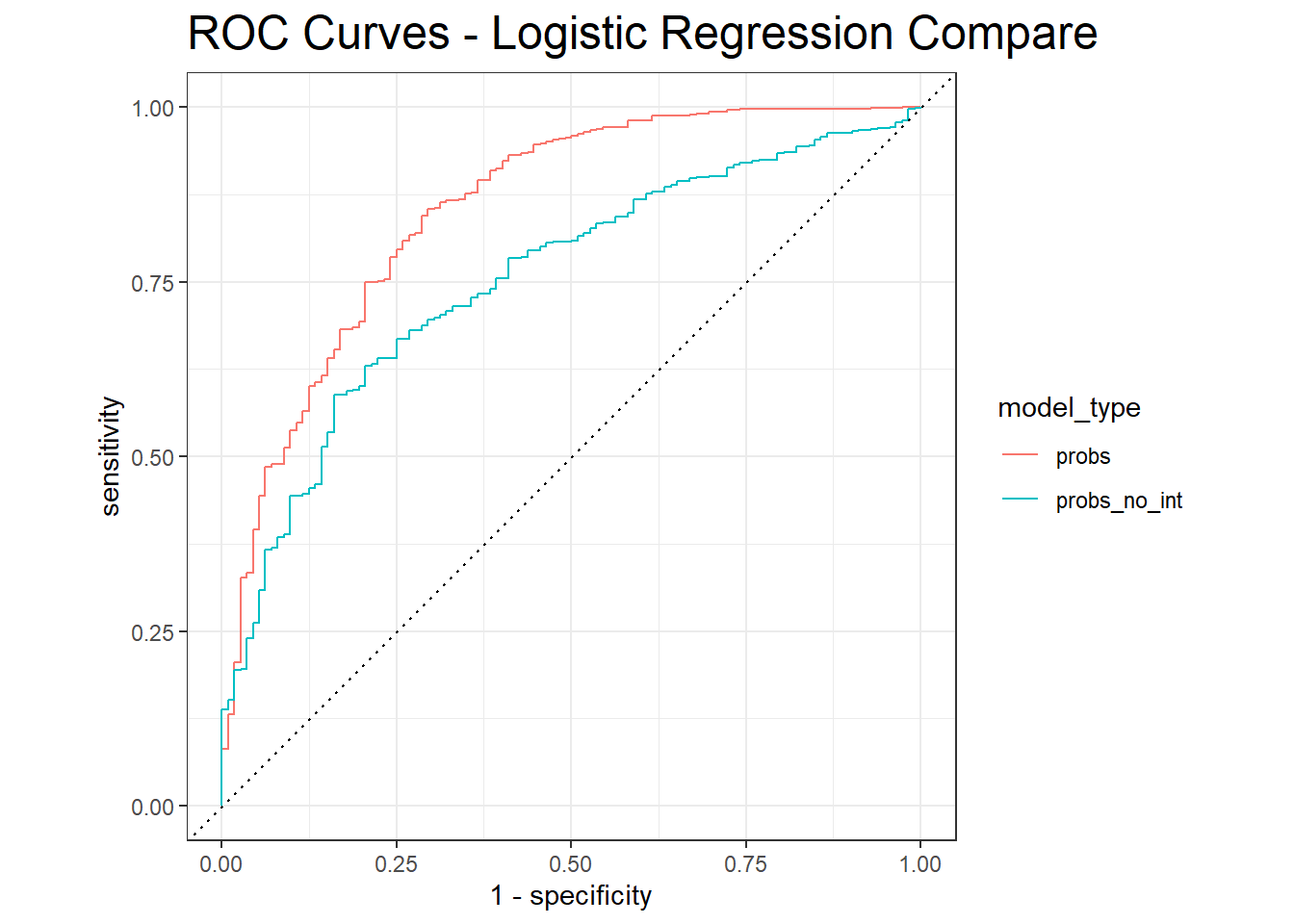
We can see that the AUC of the first model is larger, additionally, the ROC curve of the second model is below the first, therefore the first model is the better choice.
12 Strengths & Weaknesses
| Strengths | Weakness |
|---|---|
| very common and standard approach | strong assumptions about data |
| easy to understand and interpret | model form must be specified in advance |
| flexibility, can be adopted for many situations | does not handle missing data |
| provides estimates of both size and strength of the relationships among features and outcome | only numeric features, categorical and strings need encodings |
| . | understanding of statistics to fully understand model |