4 Exploratory Data Analysis
4.1 Packages, Libraries, and Functions
The first step is to read in the data. This can be done with a number of functions. Some common ones in base R include:
- for reading in R RDS files:
readRDS - for reading in csv files:
read.csv
Help for functions can be found within the R terminal by use of the question mark: ?readRDS
Sometimes you may want to use newer or more specialized packages and libraries to read in or handle data. First you will need to make sure the library is installed with install.packages('readr') then you can load the library with library('readr') , and you will have access to all of the functionality withing the package.
Alternatively, you can access individual functions from libraries by using notation such as: readr::read_csv; this tells R to look in the readr package for the function read_csv. This can be useful in programming functions and packages as well as if multiple packages contain functions with the same name.
For excel files two useful packages::functions to read in excel are:
xlsx::read.xlsxreadxl::read_excel
4.2 Read in the Data
Use the arrow <- for assignments:
4.2.1 Reminders about the Data
tibble::tribble(
  ~"Variable in Data", ~"Definition", ~"Data Type",
  'seqn', 'Respondent sequence number', 'Identifier',
  'riagendr', 'Gender', 'Categorical',
  'ridageyr', 'Age in years at screening', 'Continuous / Numerical',
  'ridreth1', 'Race/Hispanic origin', 'Categorical',
  'dmdeduc2', 'Education level', 'Adults 20+  - Categorical',
  'dmdmartl', 'Marital status', 'Categorical',
  'indhhin2', 'Annual household income', 'Categorical',
  'bmxbmi', 'Body Mass Index (kg/m**2)', 'Continuous / Numerical',
  'diq010', 'Doctor diagnosed diabetes', 'Categorical',
  'lbxglu', 'Fasting Glucose (mg/dL)', 'Continuous / Numerical'
  ) |>
knitr::kable()| Variable in Data | Definition | Data Type |
|---|---|---|
| seqn | Respondent sequence number | Identifier |
| riagendr | Gender | Categorical |
| ridageyr | Age in years at screening | Continuous / Numerical |
| ridreth1 | Race/Hispanic origin | Categorical |
| dmdeduc2 | Education level | Adults 20+ - Categorical |
| dmdmartl | Marital status | Categorical |
| indhhin2 | Annual household income | Categorical |
| bmxbmi | Body Mass Index (kg/m**2) | Continuous / Numerical |
| diq010 | Doctor diagnosed diabetes | Categorical |
| lbxglu | Fasting Glucose (mg/dL) | Continuous / Numerical |
4.3 Structure
The R Structure function will compactly display the internal structure of an R object, a diagnostic function and an alternative to summary.
To see help page for a function use ? before the function name, for example try: ?str
#structure command
str(diab_pop)
'data.frame': 5719 obs. of 10 variables:
$ seqn : num 83732 83733 83734 83735 83736 ...
$ riagendr: Factor w/ 2 levels "Male","Female": 1 1 1 2 2 2 1 2 1 1 ...
$ ridageyr: num 62 53 78 56 42 72 22 32 56 46 ...
$ ridreth1: Factor w/ 5 levels "MexicanAmerican",..: 3 3 3 3 4 1 4 1 4 3 ...
$ dmdeduc2: Factor w/ 5 levels "Less than 9th grade",..: 5 3 3 5 4 2 4 4 3 5 ...
$ dmdmartl: Factor w/ 6 levels "Married","Widowed",..: 1 3 1 6 3 4 5 1 3 6 ...
$ indhhin2: Factor w/ 14 levels "$0-$4,999","$5,000-$9,999",..: 10 4 5 10 NA 13 NA 6 3 3 ...
$ bmxbmi : num 27.8 30.8 28.8 42.4 20.3 28.6 28 28.2 33.6 27.6 ...
$ diq010 : Factor w/ 2 levels "Diabetes","No Diabetes": 1 2 1 2 2 2 2 2 1 2 ...
$ lbxglu : num NA 101 84 NA 84 107 95 NA NA NA ...4.4 Show the data
We can view the first 10 records in the data with the head command:
# show data
head(diab_pop,10)
seqn riagendr ridageyr ridreth1 dmdeduc2
1 83732 Male 62 Non-Hispanic White College grad or above
2 83733 Male 53 Non-Hispanic White High school graduate/GED
3 83734 Male 78 Non-Hispanic White High school graduate/GED
4 83735 Female 56 Non-Hispanic White College grad or above
5 83736 Female 42 Non-Hispanic Black Some college or AA degrees
6 83737 Female 72 MexicanAmerican Grades 9-11th
7 83741 Male 22 Non-Hispanic Black Some college or AA degrees
8 83742 Female 32 MexicanAmerican Some college or AA degrees
9 83744 Male 56 Non-Hispanic Black High school graduate/GED
10 83747 Male 46 Non-Hispanic White College grad or above
dmdmartl indhhin2 bmxbmi diq010 lbxglu
1 Married $65,000-$74,999 27.8 Diabetes NA
2 Divorced $15,000-$19,999 30.8 No Diabetes 101
3 Married $20,000-$24,999 28.8 Diabetes 84
4 Living with partner $65,000-$74,999 42.4 No Diabetes NA
5 Divorced <NA> 20.3 No Diabetes 84
6 Separated $75,000-$99,999 28.6 No Diabetes 107
7 Never married <NA> 28.0 No Diabetes 95
8 Married $25,000-$34,999 28.2 No Diabetes NA
9 Divorced $10,000-$14,999 33.6 Diabetes NA
10 Living with partner $10,000-$14,999 27.6 No Diabetes NA4.5 Libraries
To check which packages are loaded you can use:
# loaded packages
(.packages())
[1] "stats" "graphics" "grDevices" "datasets" "utils" "methods"
[7] "base" Make sure that the tidyverse and dplyr packages are installed. You can run install.packages(c('tidyverse','dplyr')) to install both.
To see which packages are installed you can use:
# which packages are installed
library()$results[,1]
[1] "abind" "Amelia" "anytime" "arsenal"
[5] "askpass" "backports" "base64enc" "bbotk"
[9] "BH" "BiocManager" "BiocVersion" "bit"
[13] "bit64" "bitops" "blob" "boot"
[17] "brew" "brio" "broom" "broom.helpers"
[21] "bslib" "cachem" "callr" "car"
[25] "carData" "cards" "caret" "caTools"
[29] "cellranger" "checkmate" "chron" "class"
[33] "classInt" "cli" "clipr" "clock"
[37] "clue" "cluster" "codetools" "colorspace"
[41] "combinat" "commonmark" "compare" "conflicted"
[45] "corrplot" "cowplot" "cpp11" "crayon"
[49] "credentials" "crosstalk" "curl" "data.table"
[53] "data.tree" "DBI" "dbplyr" "deming"
[57] "dendextend" "DEoptimR" "Deriv" "desc"
[61] "devtools" "diagram" "dials" "DiceDesign"
[65] "diffobj" "digest" "doBy" "doFuture"
[69] "doParallel" "downlit" "dplyr" "DT"
[73] "dtplyr" "e1071" "ellipse" "ellipsis"
[77] "emmeans" "estimability" "evaluate" "factoextra"
[81] "FactoMineR" "fansi" "farver" "fastmap"
[85] "flashClust" "fontawesome" "forcats" "foreach"
[89] "forecast" "foreign" "Formula" "fracdiff"
[93] "fs" "furrr" "future" "future.apply"
[97] "gam" "gargle" "GauPro" "gcookbook"
[101] "gdata" "generics" "gert" "GGally"
[105] "ggbernie" "ggbiplot" "ggdendro" "ggplot2"
[109] "ggpubr" "ggrepel" "ggsci" "ggsignif"
[113] "ggstats" "gh" "gitcreds" "glmnet"
[117] "globals" "glue" "gmodels" "googledrive"
[121] "googlesheets4" "gower" "GPArotation" "GPfit"
[125] "gplots" "grateful" "gridExtra" "gsubfn"
[129] "gtable" "gtools" "gtrendsR" "hardhat"
[133] "haven" "here" "highr" "Hmisc"
[137] "hms" "htmlTable" "htmltools" "htmlwidgets"
[141] "httpuv" "httr" "httr2" "ids"
[145] "igraph" "infer" "ini" "ipred"
[149] "ISLR" "isoband" "iterators" "jomo"
[153] "jquerylib" "jsonlite" "kableExtra" "KernSmooth"
[157] "klaR" "knitr" "labeling" "labelled"
[161] "laeken" "later" "lattice" "lava"
[165] "lazyeval" "lbfgs" "leaps" "lgr"
[169] "lhs" "LiblineaR" "lifecycle" "listenv"
[173] "lme4" "lmtest" "lubridate" "magrittr"
[177] "MASS" "Matrix" "MatrixModels" "mcr"
[181] "memoise" "mgcv" "mice" "microbenchmark"
[185] "mime" "miniUI" "minqa" "mirai"
[189] "mitml" "mitools" "mixopt" "mlbench"
[193] "mlr3" "mlr3learners" "mlr3measures" "mlr3misc"
[197] "mlr3pipelines" "mlr3tuning" "mnormt" "modeldata"
[201] "modelenv" "ModelMetrics" "modelr" "multcompView"
[205] "munsell" "mvtnorm" "nanonext" "networkD3"
[209] "NHANES" "nlme" "nloptr" "nnet"
[213] "numDeriv" "openssl" "ordinal" "otel"
[217] "pak" "palmerpenguins" "pan" "paradox"
[221] "parallelly" "parsnip" "patchwork" "pbkrtest"
[225] "pillar" "pkgbuild" "pkgconfig" "pkgdown"
[229] "pkgload" "plotrix" "plyr" "png"
[233] "polynom" "praise" "prettyunits" "pROC"
[237] "processx" "prodlim" "profvis" "progress"
[241] "progressr" "promises" "proto" "proxy"
[245] "PRROC" "ps" "psych" "purrr"
[249] "quantreg" "quarto" "questionr" "R.cache"
[253] "R.methodsS3" "R.oo" "R.utils" "R6"
[257] "ragg" "randomForest" "ranger" "RANN"
[261] "rappdirs" "rbibutils" "rcmdcheck" "RColorBrewer"
[265] "Rcpp" "RcppArmadillo" "RcppEigen" "Rdpack"
[269] "readr" "readxl" "recipes" "reformulas"
[273] "rematch" "rematch2" "remotes" "renv"
[277] "repr" "reprex" "reprtree" "reshape2"
[281] "rlang" "rmarkdown" "robslopes" "robustbase"
[285] "roxygen2" "rpart" "rpart.plot" "rprojroot"
[289] "rsample" "rsq" "RSQLite" "rstatix"
[293] "rstudioapi" "rversions" "rvest" "S7"
[297] "sass" "scales" "scatterplot3d" "selectr"
[301] "sessioninfo" "sfd" "shape" "shiny"
[305] "skimr" "slider" "sourcetools" "sp"
[309] "SparseM" "sparsevctrs" "spatial" "splitfngr"
[313] "sqldf" "SQUAREM" "stringi" "stringr"
[317] "styler" "survey" "survival" "svglite"
[321] "sys" "systemfonts" "tableone" "tailor"
[325] "testthat" "textshaping" "tibble" "tictoc"
[329] "tidymodels" "tidyr" "tidyselect" "tidyverse"
[333] "timechange" "timeDate" "tinytex" "tree"
[337] "tune" "tzdb" "ucminf" "urca"
[341] "urlchecker" "usethis" "utf8" "uuid"
[345] "vcd" "vctrs" "VIM" "viridis"
[349] "viridisLite" "vroom" "waldo" "warp"
[353] "whisker" "withr" "workflows" "workflowsets"
[357] "xfun" "xgboost" "xml2" "xopen"
[361] "xtable" "yaml" "yardstick" "zip"
[365] "zoo" "base" "boot" "class"
[369] "cluster" "codetools" "compiler" "datasets"
[373] "foreign" "graphics" "grDevices" "grid"
[377] "KernSmooth" "lattice" "MASS" "Matrix"
[381] "methods" "mgcv" "nlme" "nnet"
[385] "parallel" "rpart" "spatial" "splines"
[389] "stats" "stats4" "survival" "tcltk"
[393] "tools" "translations" "utils" # some additional informaion on the package including the version
tibble::as_tibble(installed.packages())# A tibble: 395 × 17
Package LibPath Version Priority Depends Imports LinkingTo Suggests Enhances
<chr> <chr> <chr> <chr> <chr> <chr> <chr> <chr> <chr>
1 abind C:/Use… 1.4-8 <NA> R (>= … "metho… <NA> <NA> <NA>
2 Amelia C:/Use… 1.8.3 <NA> R (>= … "forei… Rcpp (>=… "tcltk,… <NA>
3 anytime C:/Use… 0.3.13 <NA> R (>= … "Rcpp … Rcpp (>=… "tinyte… <NA>
4 arsenal C:/Use… 3.6.3 <NA> R (>= … "knitr… <NA> "broom … <NA>
5 askpass C:/Use… 1.2.1 <NA> <NA> "sys (… <NA> "testth… <NA>
6 backpor… C:/Use… 1.5.1 <NA> R (>= … <NA> <NA> <NA> <NA>
7 base64e… C:/Use… 0.1-6 <NA> R (>= … <NA> <NA> <NA> png
8 bbotk C:/Use… 1.10.0 <NA> parado… "check… <NA> "adagio… <NA>
9 BH C:/Use… 1.90.0… <NA> <NA> <NA> <NA> <NA> <NA>
10 BiocMan… C:/Use… 1.30.27 <NA> <NA> "utils" <NA> "BiocVe… <NA>
# ℹ 385 more rows
# ℹ 8 more variables: License <chr>, License_is_FOSS <chr>,
# License_restricts_use <chr>, OS_type <chr>, MD5sum <chr>,
# NeedsCompilation <chr>, Built <chr>, Published <chr>The following function will check if a list of packages are already installed, if not then it will install them:
# install package if missing
install_if_not <- function( list.of.packages ) {

  new.packages <- list.of.packages[!(list.of.packages %in% installed.packages()[,"Package"])]

  if(length(new.packages)) { pak::pak(new.packages) }
  else { print(paste0("the package '", list.of.packages , "' is already installed")) }
}
You can use the function like this:
# test function
install_if_not(c("caret","randomForest"))
[1] "the package 'caret' is already installed"
[2] "the package 'randomForest' is already installed"We make sections of code accessible to installed packages by using library command:
Attaching package: 'dplyr'The following objects are masked from 'package:stats':
filter, lagThe following objects are masked from 'package:base':
intersect, setdiff, setequal, unionglimpse(diab_pop)Rows: 5,719
Columns: 10
$ seqn <dbl> 83732, 83733, 83734, 83735, 83736, 83737, 83741, 83742, 83744…
$ riagendr <fct> Male, Male, Male, Female, Female, Female, Male, Female, Male,…
$ ridageyr <dbl> 62, 53, 78, 56, 42, 72, 22, 32, 56, 46, 45, 30, 67, 67, 57, 8…
$ ridreth1 <fct> Non-Hispanic White, Non-Hispanic White, Non-Hispanic White, N…
$ dmdeduc2 <fct> College grad or above, High school graduate/GED, High school …
$ dmdmartl <fct> Married, Divorced, Married, Living with partner, Divorced, Se…
$ indhhin2 <fct> "$65,000-$74,999", "$15,000-$19,999", "$20,000-$24,999", "$65…
$ bmxbmi <dbl> 27.8, 30.8, 28.8, 42.4, 20.3, 28.6, 28.0, 28.2, 33.6, 27.6, 2…
$ diq010 <fct> Diabetes, No Diabetes, Diabetes, No Diabetes, No Diabetes, No…
$ lbxglu <dbl> NA, 101, 84, NA, 84, 107, 95, NA, NA, NA, 84, NA, 130, 284, 3…(.packages())[1] "dplyr" "stats" "graphics" "grDevices" "datasets" "utils"
[7] "methods" "base" [1] "dplyr"detach(package:dplyr)
#the dplyr package has now been detached. calls to functions may have errorsAdditionally, we can access a function from a library without loading the entire library, this can be done by using a command such as package::function. This notation is needed in any instance where two or more loaded packages have at least one function with the same name. This notation is also useful in development of functions and packages.
For instance, the glimpse function from the dplyr package can also be accessed by using the following command
# glimpse the data
dplyr::glimpse(diab_pop)
Rows: 5,719
Columns: 10
$ seqn <dbl> 83732, 83733, 83734, 83735, 83736, 83737, 83741, 83742, 83744…
$ riagendr <fct> Male, Male, Male, Female, Female, Female, Male, Female, Male,…
$ ridageyr <dbl> 62, 53, 78, 56, 42, 72, 22, 32, 56, 46, 45, 30, 67, 67, 57, 8…
$ ridreth1 <fct> Non-Hispanic White, Non-Hispanic White, Non-Hispanic White, N…
$ dmdeduc2 <fct> College grad or above, High school graduate/GED, High school …
$ dmdmartl <fct> Married, Divorced, Married, Living with partner, Divorced, Se…
$ indhhin2 <fct> "$65,000-$74,999", "$15,000-$19,999", "$20,000-$24,999", "$65…
$ bmxbmi <dbl> 27.8, 30.8, 28.8, 42.4, 20.3, 28.6, 28.0, 28.2, 33.6, 27.6, 2…
$ diq010 <fct> Diabetes, No Diabetes, Diabetes, No Diabetes, No Diabetes, No…
$ lbxglu <dbl> NA, 101, 84, NA, 84, 107, 95, NA, NA, NA, 84, NA, 130, 284, 3…And just notice that without the library loaded or the dplyr:: in front we can error:
# error
glimpse(diab_pop)
Error in `glimpse()`:
! could not find function "glimpse"A Tibble is an more modern R version of a dataframe, you can easily convert a dataframe to a tibble.
tibble::as_tibble(diab_pop)# A tibble: 5,719 × 10
seqn riagendr ridageyr ridreth1 dmdeduc2 dmdmartl indhhin2 bmxbmi diq010
<dbl> <fct> <dbl> <fct> <fct> <fct> <fct> <dbl> <fct>
1 83732 Male 62 Non-Hispani… College… Married $65,000… 27.8 Diabe…
2 83733 Male 53 Non-Hispani… High sc… Divorced $15,000… 30.8 No Di…
3 83734 Male 78 Non-Hispani… High sc… Married $20,000… 28.8 Diabe…
4 83735 Female 56 Non-Hispani… College… Living … $65,000… 42.4 No Di…
5 83736 Female 42 Non-Hispani… Some co… Divorced <NA> 20.3 No Di…
6 83737 Female 72 MexicanAmer… Grades … Separat… $75,000… 28.6 No Di…
7 83741 Male 22 Non-Hispani… Some co… Never m… <NA> 28 No Di…
8 83742 Female 32 MexicanAmer… Some co… Married $25,000… 28.2 No Di…
9 83744 Male 56 Non-Hispani… High sc… Divorced $10,000… 33.6 Diabe…
10 83747 Male 46 Non-Hispani… College… Living … $10,000… 27.6 No Di…
# ℹ 5,709 more rows
# ℹ 1 more variable: lbxglu <dbl>
4.6 summary
The summary is a generic function used to produce result summaries of the results of various model fitting functions. See ?summary for more information.
summary(diab_pop) seqn riagendr ridageyr ridreth1
Min. :83732 Male :2747 Min. :20.00 MexicanAmerican : 995
1st Qu.:86171 Female:2972 1st Qu.:34.00 Other Hispanic : 768
Median :88651 Median :49.00 Non-Hispanic White:1863
Mean :88672 Mean :49.54 Non-Hispanic Black:1198
3rd Qu.:91166 3rd Qu.:64.00 Other : 895
Max. :93702 Max. :80.00
dmdeduc2 dmdmartl
Less than 9th grade : 688 Married :2886
Grades 9-11th : 676 Widowed : 421
High school graduate/GED :1236 Divorced : 614
Some college or AA degrees:1692 Separated : 192
College grad or above :1422 Never married :1048
NAs : 5 Living with partner: 555
NAs : 3
indhhin2 bmxbmi diq010 lbxglu
$100,000+ : 910 Min. :14.50 Diabetes : 844 Min. : 21.0
$25,000-$34,999: 596 1st Qu.:24.50 No Diabetes:4875 1st Qu.: 95.0
$75,000-$99,999: 524 Median :28.50 Median :103.0
$45,000-$54,999: 451 Mean :29.54 Mean :113.6
$20,000-$24,999: 350 3rd Qu.:33.20 3rd Qu.:114.0
(Other) :1590 Max. :67.30 Max. :479.0
NAs :1298 NAs :313 NAs :3267 by(diab_pop, diab_pop$diq010, summary)diab_pop$diq010: Diabetes
seqn riagendr ridageyr ridreth1
Min. :83732 Male :456 Min. :21.00 MexicanAmerican :200
1st Qu.:86069 Female:388 1st Qu.:53.00 Other Hispanic :119
Median :88610 Median :63.00 Non-Hispanic White:217
Mean :88574 Mean :61.34 Non-Hispanic Black:203
3rd Qu.:90995 3rd Qu.:71.00 Other :105
Max. :93689 Max. :80.00
dmdeduc2 dmdmartl
Less than 9th grade :161 Married :471
Grades 9-11th :123 Widowed :100
High school graduate/GED :185 Divorced :106
Some college or AA degrees:229 Separated : 29
College grad or above :145 Never married : 83
NAs : 1 Living with partner: 55
indhhin2 bmxbmi diq010 lbxglu
$100,000+ : 89 Min. :16.0 Diabetes :844 Min. : 21
$25,000-$34,999: 86 1st Qu.:27.4 No Diabetes: 0 1st Qu.:117
$10,000-$14,999: 81 Median :31.4 Median :147
$20,000-$24,999: 68 Mean :32.6 Mean :166
$45,000-$54,999: 65 3rd Qu.:36.3 3rd Qu.:192
(Other) :261 Max. :67.3 Max. :479
NAs :194 NAs :55 NAs :462
------------------------------------------------------------
diab_pop$diq010: No Diabetes
seqn riagendr ridageyr ridreth1
Min. :83733 Male :2291 Min. :20.00 MexicanAmerican : 795
1st Qu.:86190 Female:2584 1st Qu.:32.00 Other Hispanic : 649
Median :88654 Median :46.00 Non-Hispanic White:1646
Mean :88689 Mean :47.49 Non-Hispanic Black: 995
3rd Qu.:91193 3rd Qu.:61.00 Other : 790
Max. :93702 Max. :80.00
dmdeduc2 dmdmartl
Less than 9th grade : 527 Married :2415
Grades 9-11th : 553 Widowed : 321
High school graduate/GED :1051 Divorced : 508
Some college or AA degrees:1463 Separated : 163
College grad or above :1277 Never married : 965
NAs : 4 Living with partner: 500
NAs : 3
indhhin2 bmxbmi diq010 lbxglu
$100,000+ : 821 Min. :14.50 Diabetes : 0 Min. : 64.0
$25,000-$34,999: 510 1st Qu.:24.10 No Diabetes:4875 1st Qu.: 94.0
$75,000-$99,999: 472 Median :28.00 Median :101.0
$45,000-$54,999: 386 Mean :29.02 Mean :103.9
$15,000-$19,999: 290 3rd Qu.:32.50 3rd Qu.:109.0
(Other) :1292 Max. :64.60 Max. :397.0
NAs :1104 NAs :258 NAs :2805 4.7 Missing Data
4.7.1 Amelia
4.7.2 Mice
install_if_not("mice")[1] "the package 'mice' is already installed"install_if_not("VIM")[1] "the package 'VIM' is already installed"install_if_not("lattice")[1] "the package 'lattice' is already installed"
Attaching package: 'mice'The following object is masked from 'package:stats':
filterThe following objects are masked from 'package:base':
cbind, rbindLoading required package: colorspaceLoading required package: gridRegistered S3 method overwritten by 'car':
method from
na.action.merMod lme4VIM is ready to use.Suggestions and bug-reports can be submitted at: https://github.com/statistikat/VIM/issues
Attaching package: 'VIM'The following object is masked from 'package:datasets':
sleeplibrary(lattice)
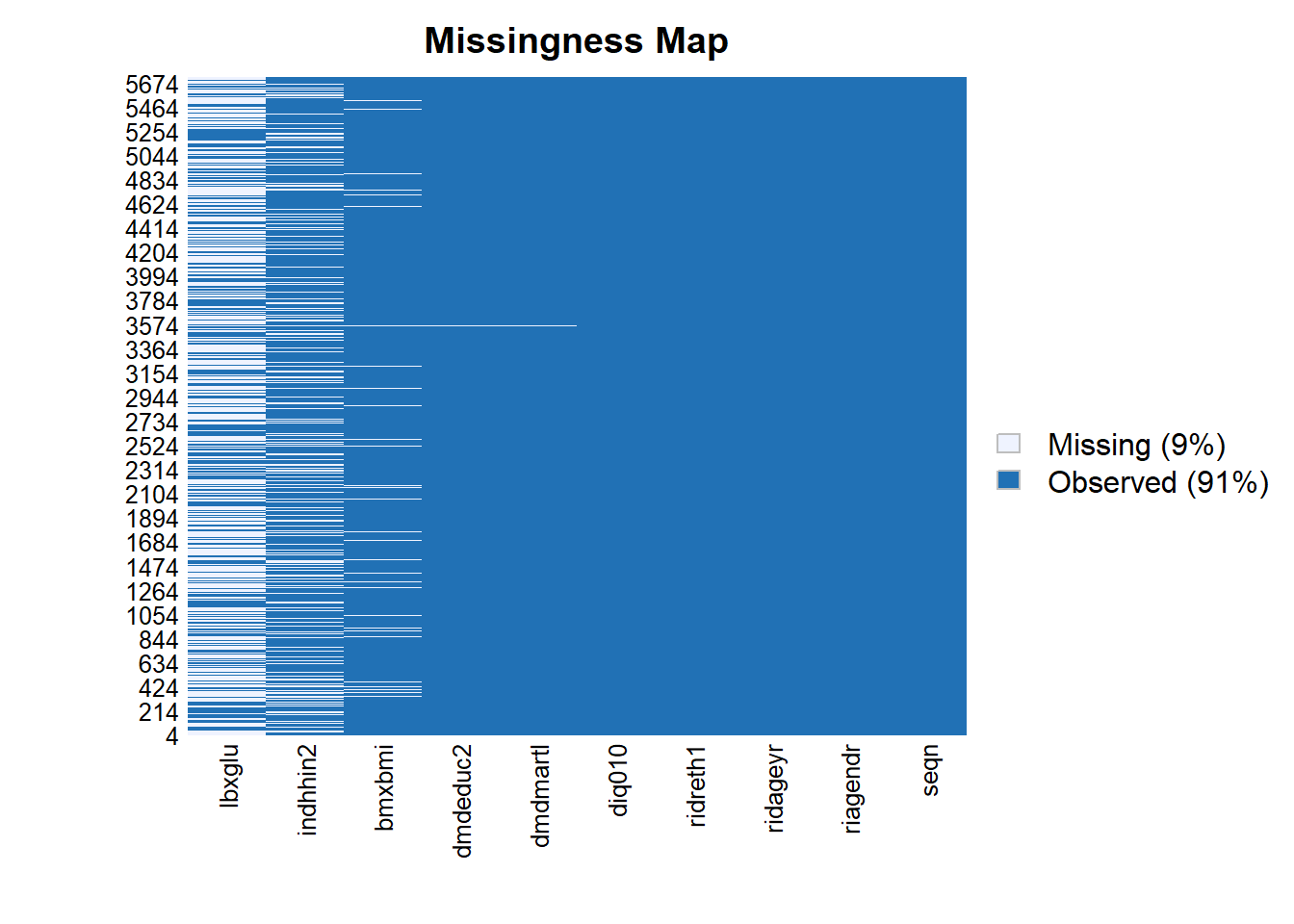
#understand the missing value pattern
md.pattern(diab_pop)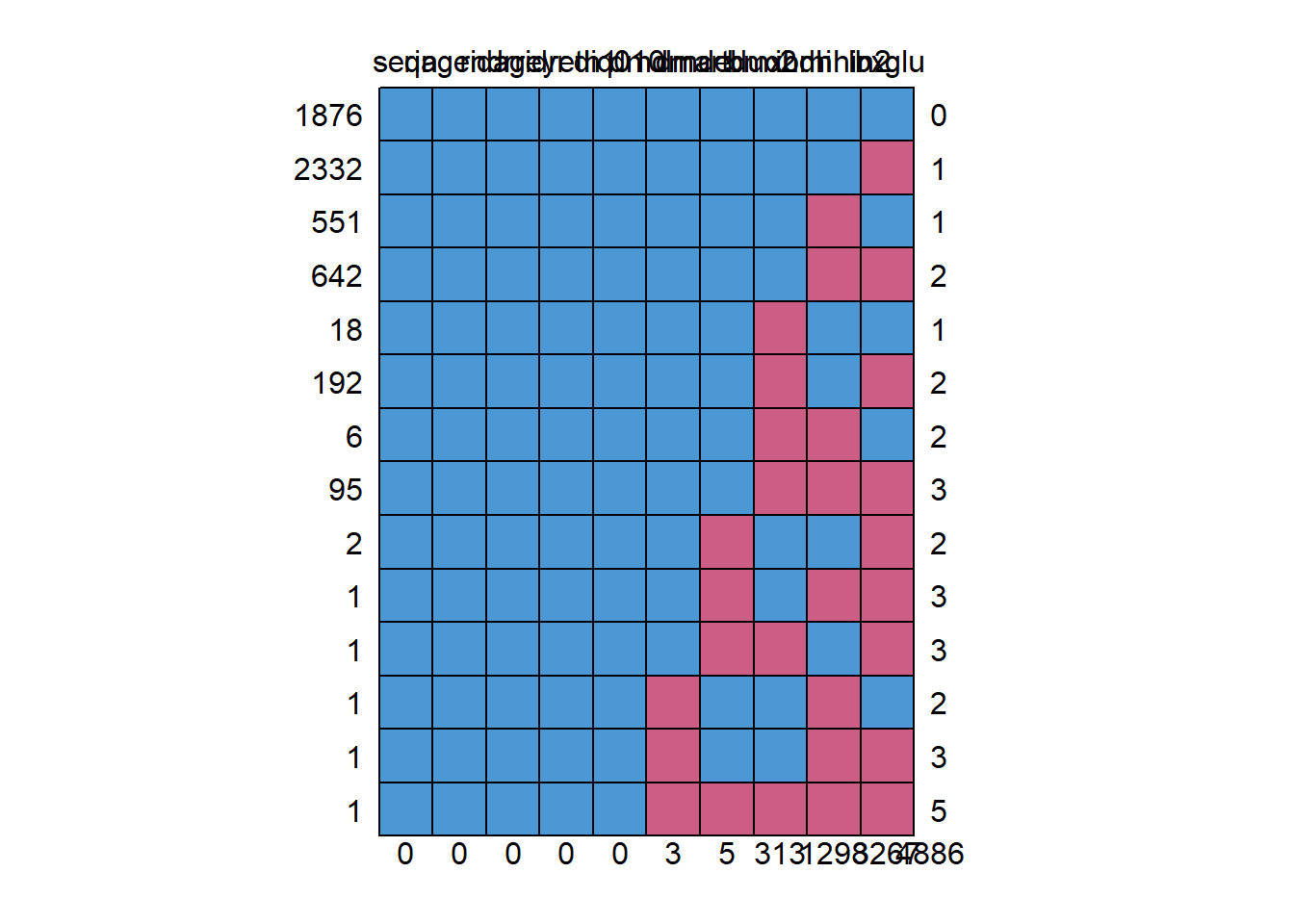
     seqn riagendr ridageyr ridreth1 diq010 dmdmartl dmdeduc2 bmxbmi indhhin2
1876    1        1        1        1      1        1        1      1        1
2332    1        1        1        1      1        1        1      1        1
551     1        1        1        1      1        1        1      1        0
642     1        1        1        1      1        1        1      1        0
18      1        1        1        1      1        1        1      0        1
192     1        1        1        1      1        1        1      0        1
6       1        1        1        1      1        1        1      0        0
95      1        1        1        1      1        1        1      0        0
2       1        1        1        1      1        1        0      1        1
1       1        1        1        1      1        1        0      1        0
1       1        1        1        1      1        1        0      0        1
1       1        1        1        1      1        0        1      1        0
1       1        1        1        1      1        0        1      1        0
1       1        1        1        1      1        0        0      0        0
        0        0        0        0      0        3        5    313     1298
     lbxglu
1876      1    0
2332      0    1
551       1    1
642       0    2
18        1    1
192       0    2
6         1    2
95        0    3
2         0    2
1         0    3
1         0    3
1         1    2
1         0    3
1         0    5
3267 4886Warning in plot.aggr(res, ...): not enough horizontal space to display
frequencies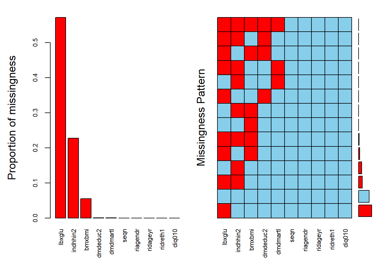
 Variables sorted by number of missings:
 Variable        Count
   lbxglu 0.5712537157
 indhhin2 0.2269627557
   bmxbmi 0.0547298479
 dmdeduc2 0.0008742787
 dmdmartl 0.0005245672
     seqn 0.0000000000
 riagendr 0.0000000000
 ridageyr 0.0000000000
 ridreth1 0.0000000000
   diq010 0.0000000000
#Drawing margin plot
marginplot(diab_pop[, c("lbxglu", "diq010")],
cex.numbers = 1.2,
pch = 19)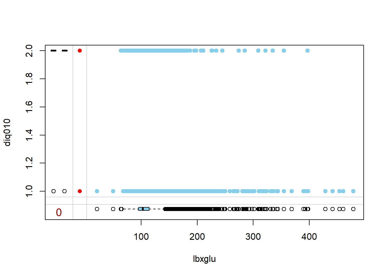
4.8 sqldf
You can also create summary tables with sql and the sqldf:
install_if_not('sqldf')[1] "the package 'sqldf' is already installed"# Average age by Diabetes
sqldf::sqldf('select diq010,
avg(ridageyr) as mean_age
from diab_pop
group by diq010
order by diq010') diq010 mean_age
1 Diabetes 61.33768
2 No Diabetes 47.49313'data.frame': 4 obs. of 3 variables:
$ diq010 : Factor w/ 2 levels "Diabetes","No Diabetes": 2 2 1 1
$ riagendr: Factor w/ 2 levels "Male","Female": 2 1 1 2
$ cnt : int 2584 2291 456 388T_sqldf diq010 riagendr cnt
1 No Diabetes Female 2584
2 No Diabetes Male 2291
3 Diabetes Male 456
4 Diabetes Female 388
4.9 dplyr
dplyr is a popular package to manage many common data manipulation tasks and data summaries.
Attaching package: 'dplyr'The following objects are masked from 'package:stats':
filter, lagThe following objects are masked from 'package:base':
intersect, setdiff, setequal, union# A tibble: 2 × 2
diq010 mean_age
<fct> <dbl>
1 Diabetes 61.3
2 No Diabetes 47.5`summarise()` has regrouped the output.
ℹ Summaries were computed grouped by diq010 and riagendr.
ℹ Output is grouped by diq010.
ℹ Use `summarise(.groups = "drop_last")` to silence this message.
ℹ Use `summarise(.by = c(diq010, riagendr))` for per-operation grouping
(`?dplyr::dplyr_by`) instead.str(T_dplyr_dm2_gender)tibble [4 × 3] (S3: tbl_df/tbl/data.frame)
$ diq010 : Factor w/ 2 levels "Diabetes","No Diabetes": 2 2 1 1
$ riagendr: Factor w/ 2 levels "Male","Female": 2 1 1 2
$ cnt : int [1:4] 2584 2291 456 388T_dplyr_dm2_gender # A tibble: 4 × 3
diq010 riagendr cnt
<fct> <fct> <int>
1 No Diabetes Female 2584
2 No Diabetes Male 2291
3 Diabetes Male 456
4 Diabetes Female 388
4.9.1 Additional dplyr resources
- What is
dplyr: https://dplyr.tidyverse.org/ - Introduction to
dplyrvignette: https://cran.r-project.org/web/packages/dplyr/vignettes/dplyr.html -
dplyrcheatsheet: https://github.com/rstudio/cheatsheets/blob/master/data-transformation.pdf
4.10 comparedf
The comparedf function in the arsenal package can be used to compare two data-frames:
install_if_not('arsenal')[1] "the package 'arsenal' is already installed"my_comparison <- arsenal::comparedf(T_sqldf , T_dplyr_dm2_gender)
my_comparisonCompare Object
Function Call:
arsenal::comparedf(x = T_sqldf, y = T_dplyr_dm2_gender)
Shared: 3 non-by variables and 4 observations.
Not shared: 0 variables and 0 observations.
Differences found in 0/3 variables compared.
0 variables compared have non-identical attributes.summary(my_comparison)
Table: Summary of data.frames
version arg ncol nrow
-------- ------------------- ----- -----
x T_sqldf 3 4
y T_dplyr_dm2_gender 3 4
Table: Summary of overall comparison
statistic value
------------------------------------------------------------ ------
Number of by-variables 0
Number of non-by variables in common 3
Number of variables compared 3
Number of variables in x but not y 0
Number of variables in y but not x 0
Number of variables compared with some values unequal 0
Number of variables compared with all values equal 3
Number of observations in common 4
Number of observations in x but not y 0
Number of observations in y but not x 0
Number of observations with some compared variables unequal 0
Number of observations with all compared variables equal 4
Number of values unequal 0
Table: Variables not shared
------------------------
No variables not shared
------------------------
Table: Other variables not compared
--------------------------------
No other variables not compared
--------------------------------
Table: Observations not shared
---------------------------
No observations not shared
---------------------------
Table: Differences detected by variable
var.x var.y n NAs
--------- --------- --- ----
diq010 diq010 0 0
riagendr riagendr 0 0
cnt cnt 0 0
Table: Differences detected
------------------------
No differences detected
------------------------
Table: Non-identical attributes
----------------------------
No non-identical attributes
----------------------------str(my_comparison)List of 4
$ frame.summary:Classes 'comparedf.frame.summary' and 'data.frame': 2 obs. of 8 variables:
..$ version : chr [1:2] "x" "y"
..$ arg : chr [1:2] "T_sqldf" "T_dplyr_dm2_gender"
..$ ncol : int [1:2] 3 3
..$ nrow : int [1:2] 4 4
..$ by :List of 2
.. ..$ : chr "..row.names.."
.. ..$ : chr "..row.names.."
.. ..- attr(*, "byrow")= logi TRUE
..$ attrs :List of 2
.. ..$ :List of 3
.. .. ..$ names : chr [1:3] "diq010" "riagendr" "cnt"
.. .. ..$ row.names: int [1:4] 1 2 3 4
.. .. ..$ class : chr "data.frame"
.. ..$ :List of 3
.. .. ..$ names : chr [1:3] "diq010" "riagendr" "cnt"
.. .. ..$ row.names: int [1:4] 1 2 3 4
.. .. ..$ class : chr [1:3] "tbl_df" "tbl" "data.frame"
..$ unique :List of 2
.. ..$ :'data.frame': 0 obs. of 2 variables:
.. .. ..$ ..row.names..: int(0)
.. .. ..$ observation : int(0)
.. ..$ :'data.frame': 0 obs. of 2 variables:
.. .. ..$ ..row.names..: int(0)
.. .. ..$ observation : int(0)
..$ n.shared: int [1:2] 4 4
$ vars.summary :Classes 'comparedf.vars.summary' and 'data.frame': 4 obs. of 8 variables:
..$ var.x : chr [1:4] "diq010" "riagendr" "cnt" "..row.names.."
..$ pos.x : int [1:4] 1 2 3 4
..$ class.x:List of 4
.. ..$ : chr "factor"
.. ..$ : chr "factor"
.. ..$ : chr "integer"
.. ..$ : chr "integer"
..$ var.y : chr [1:4] "diq010" "riagendr" "cnt" "..row.names.."
..$ pos.y : int [1:4] 1 2 3 4
..$ class.y:List of 4
.. ..$ : chr "factor"
.. ..$ : chr "factor"
.. ..$ : chr "integer"
.. ..$ : chr "integer"
..$ values :List of 4
.. ..$ :'data.frame': 0 obs. of 5 variables:
.. .. ..$ ..row.names..: int(0)
.. .. ..$ values.x : Factor w/ 2 levels "Diabetes","No Diabetes":
.. .. ..$ values.y : Factor w/ 2 levels "Diabetes","No Diabetes":
.. .. ..$ row.x : int(0)
.. .. ..$ row.y : int(0)
.. ..$ :'data.frame': 0 obs. of 5 variables:
.. .. ..$ ..row.names..: int(0)
.. .. ..$ values.x : Factor w/ 2 levels "Male","Female":
.. .. ..$ values.y : Factor w/ 2 levels "Male","Female":
.. .. ..$ row.x : int(0)
.. .. ..$ row.y : int(0)
.. ..$ :'data.frame': 0 obs. of 5 variables:
.. .. ..$ ..row.names..: int(0)
.. .. ..$ values.x : 'AsIs' int(0)
.. .. ..$ values.y : 'AsIs' int(0)
.. .. ..$ row.x : int(0)
.. .. ..$ row.y : int(0)
.. ..$ : chr "by-variable"
..$ attrs :List of 4
.. ..$ :'data.frame': 0 obs. of 3 variables:
.. .. ..$ name : chr(0)
.. .. ..$ attr.x: Named list()
.. .. ..$ attr.y: Named list()
.. ..$ :'data.frame': 0 obs. of 3 variables:
.. .. ..$ name : chr(0)
.. .. ..$ attr.x: Named list()
.. .. ..$ attr.y: Named list()
.. ..$ : NULL
.. ..$ : NULL
$ control :List of 16
..$ tol.logical :List of 1
.. ..$ :function (x, y)
..$ tol.num :List of 1
.. ..$ :function (x, y, tol)
..$ tol.num.val : num 1.49e-08
..$ int.as.num : logi FALSE
..$ tol.char :List of 1
.. ..$ :function (x, y)
..$ tol.factor :List of 1
.. ..$ :function (x, y)
..$ factor.as.char : logi FALSE
..$ tol.date :List of 1
.. ..$ :function (x, y, tol)
..$ tol.date.val : num 0
..$ tol.other :List of 1
.. ..$ :function (x, y)
..$ tol.vars : chr "none"
..$ max.print.vars : logi NA
..$ max.print.obs : logi NA
..$ max.print.diffs.per.var: num 10
..$ max.print.diffs : num 50
..$ max.print.attrs : logi NA
$ Call : language arsenal::comparedf(x = T_sqldf, y = T_dplyr_dm2_gender)
- attr(*, "class")= chr "comparedf"4.11 Chi Square Test
# The table command can give us a table of counts of categorical columns:
table(diab_pop$diq010, diab_pop$riagendr)
Male Female
Diabetes 456 388
No Diabetes 2291 2584table(diab_pop$dmdmartl, diab_pop$riagendr, diab_pop$diq010), , = Diabetes
Male Female
Married 299 172
Widowed 30 70
Divorced 46 60
Separated 11 18
Never married 39 44
Living with partner 31 24
, , = No Diabetes
Male Female
Married 1229 1186
Widowed 79 242
Divorced 200 308
Separated 58 105
Never married 471 494
Living with partner 253 247# We can use similar call for the chi square test:
chisq.test(diab_pop$diq010, diab_pop$riagendr)
Pearson's Chi-squared test with Yates' continuity correction
data: diab_pop$diq010 and diab_pop$riagendr
X-squared = 13.978, df = 1, p-value = 0.0001849# We can store the results and then use them:
table.sex_dm2 <- table(diab_pop$riagendr, diab_pop$diq010)
table.sex_dm2
Diabetes No Diabetes
Male 456 2291
Female 388 2584chisq.test(table.sex_dm2)
Pearson's Chi-squared test with Yates' continuity correction
data: table.sex_dm2
X-squared = 13.978, df = 1, p-value = 0.00018494.11.1 Use the output
The R functions can have multiple outputs. We can also see other data associated with the output, the structure command can be used to help:
chisq_results <- chisq.test(diab_pop$diq010, diab_pop$riagendr)
str(chisq_results)List of 9
$ statistic: Named num 14
..- attr(*, "names")= chr "X-squared"
$ parameter: Named int 1
..- attr(*, "names")= chr "df"
$ p.value : num 0.000185
$ method : chr "Pearson's Chi-squared test with Yates' continuity correction"
$ data.name: chr "diab_pop$diq010 and diab_pop$riagendr"
$ observed : 'table' int [1:2, 1:2] 456 2291 388 2584
..- attr(*, "dimnames")=List of 2
.. ..$ diab_pop$diq010 : chr [1:2] "Diabetes" "No Diabetes"
.. ..$ diab_pop$riagendr: chr [1:2] "Male" "Female"
$ expected : num [1:2, 1:2] 405 2342 439 2533
..- attr(*, "dimnames")=List of 2
.. ..$ diab_pop$diq010 : chr [1:2] "Diabetes" "No Diabetes"
.. ..$ diab_pop$riagendr: chr [1:2] "Male" "Female"
$ residuals: 'table' num [1:2, 1:2] 2.51 -1.05 -2.42 1.01
..- attr(*, "dimnames")=List of 2
.. ..$ diab_pop$diq010 : chr [1:2] "Diabetes" "No Diabetes"
.. ..$ diab_pop$riagendr: chr [1:2] "Male" "Female"
$ stdres : 'table' num [1:2, 1:2] 3.78 -3.78 -3.78 3.78
..- attr(*, "dimnames")=List of 2
.. ..$ diab_pop$diq010 : chr [1:2] "Diabetes" "No Diabetes"
.. ..$ diab_pop$riagendr: chr [1:2] "Male" "Female"
- attr(*, "class")= chr "htest"# We can access different portions of the output:
chisq_results$p.value[1] 0.0001849292chisq_results$statisticX-squared
13.97834 chisq_results$method[1] "Pearson's Chi-squared test with Yates' continuity correction"
4.11.2 broom
The default output of the chisq.test test is a list, the tidy function in the broom package will take many results from other packages and convert into tibbles for easier handling:
str(chisq_results)List of 9
$ statistic: Named num 14
..- attr(*, "names")= chr "X-squared"
$ parameter: Named int 1
..- attr(*, "names")= chr "df"
$ p.value : num 0.000185
$ method : chr "Pearson's Chi-squared test with Yates' continuity correction"
$ data.name: chr "diab_pop$diq010 and diab_pop$riagendr"
$ observed : 'table' int [1:2, 1:2] 456 2291 388 2584
..- attr(*, "dimnames")=List of 2
.. ..$ diab_pop$diq010 : chr [1:2] "Diabetes" "No Diabetes"
.. ..$ diab_pop$riagendr: chr [1:2] "Male" "Female"
$ expected : num [1:2, 1:2] 405 2342 439 2533
..- attr(*, "dimnames")=List of 2
.. ..$ diab_pop$diq010 : chr [1:2] "Diabetes" "No Diabetes"
.. ..$ diab_pop$riagendr: chr [1:2] "Male" "Female"
$ residuals: 'table' num [1:2, 1:2] 2.51 -1.05 -2.42 1.01
..- attr(*, "dimnames")=List of 2
.. ..$ diab_pop$diq010 : chr [1:2] "Diabetes" "No Diabetes"
.. ..$ diab_pop$riagendr: chr [1:2] "Male" "Female"
$ stdres : 'table' num [1:2, 1:2] 3.78 -3.78 -3.78 3.78
..- attr(*, "dimnames")=List of 2
.. ..$ diab_pop$diq010 : chr [1:2] "Diabetes" "No Diabetes"
.. ..$ diab_pop$riagendr: chr [1:2] "Male" "Female"
- attr(*, "class")= chr "htest"install_if_not('broom')[1] "the package 'broom' is already installed"tibble [1 × 4] (S3: tbl_df/tbl/data.frame)
$ statistic: Named num 14
..- attr(*, "names")= chr "X-squared"
$ p.value : num 0.000185
$ parameter: Named int 1
..- attr(*, "names")= chr "df"
$ method : chr "Pearson's Chi-squared test with Yates' continuity correction"tidy_chisq_results$p.value[1] 0.00018492924.11.3 Some Example Plots
We can also make some basic graphics that are in base R:
plot(table.sex_dm2)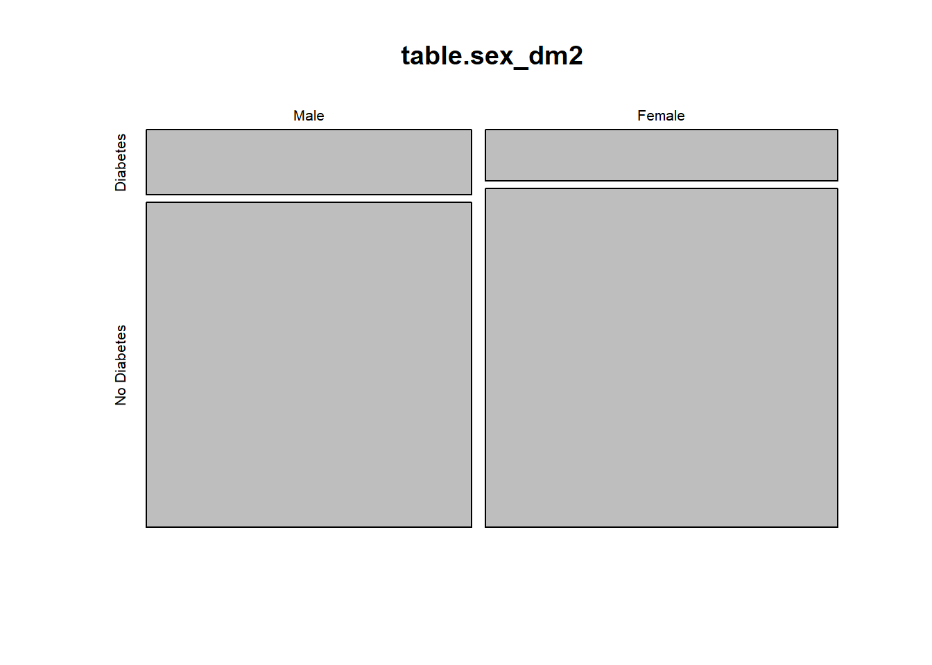
mosaicplot(table.sex_dm2,
main = "Diabetes by Sex Mosaic Plot",
xlab = "Sex",
ylab = "Diabetes",
las = 1,
border = "chocolate",
shade = TRUE) 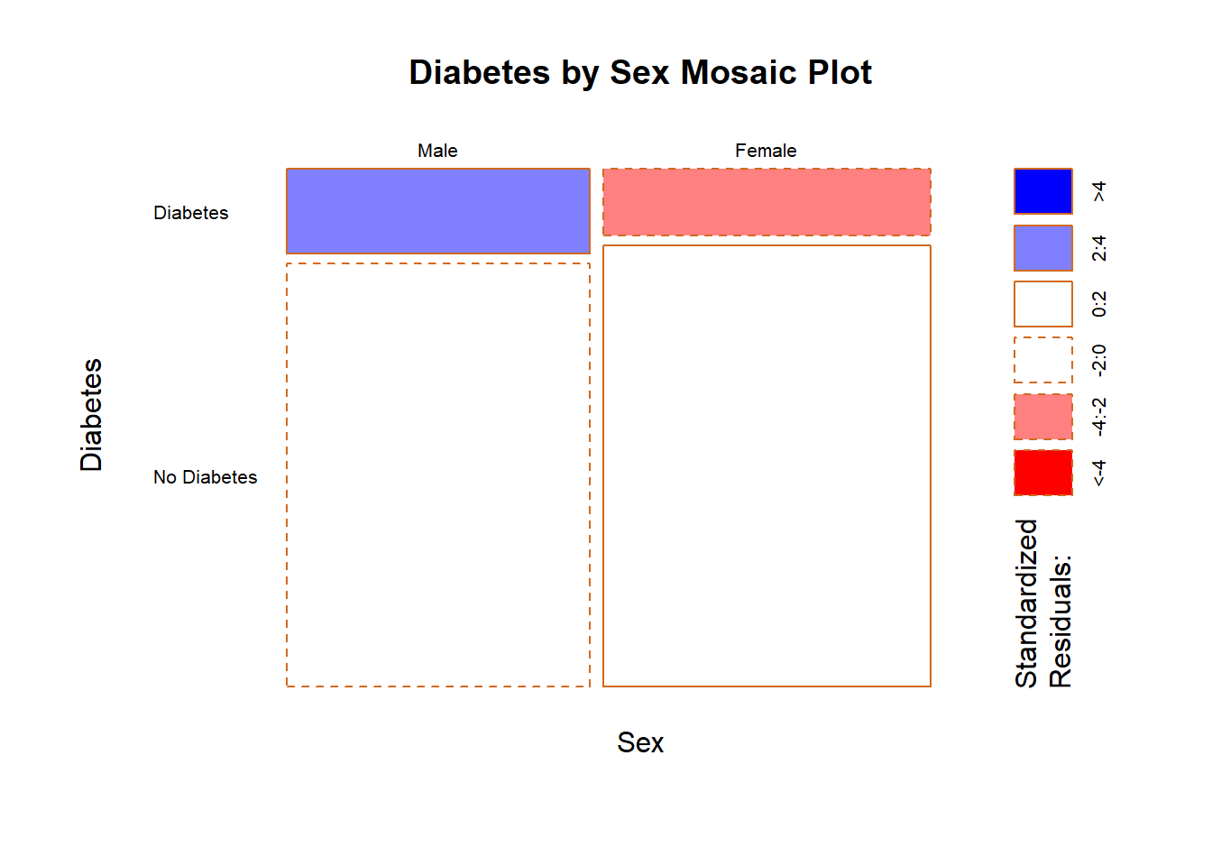
Other graphics are accessible by installing various packages:
4.11.4 ggplot2
4.11.5 gplots
install_if_not('gplots')[1] "the package 'gplots' is already installed"gplots::balloonplot(table.sex_dm2,
main ="Balloon Plot for Sex by Diabetes \n Area is proportional to Freq.")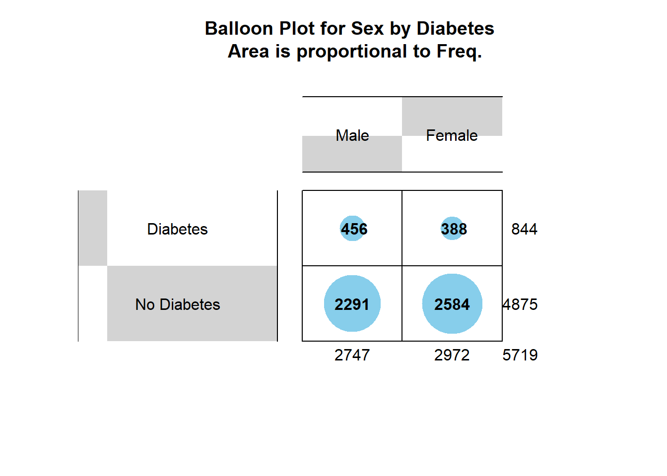
4.11.6 corrplot
We can view the residuals from the chi-square test:
chisq_results$residuals diab_pop$riagendr
diab_pop$diq010 Male Female
Diabetes 2.513228 -2.416222
No Diabetes -1.045721 1.005358install_if_not('corrplot')[1] "the package 'corrplot' is already installed"corrplot::corrplot(chisq_results$residuals, is.cor = FALSE)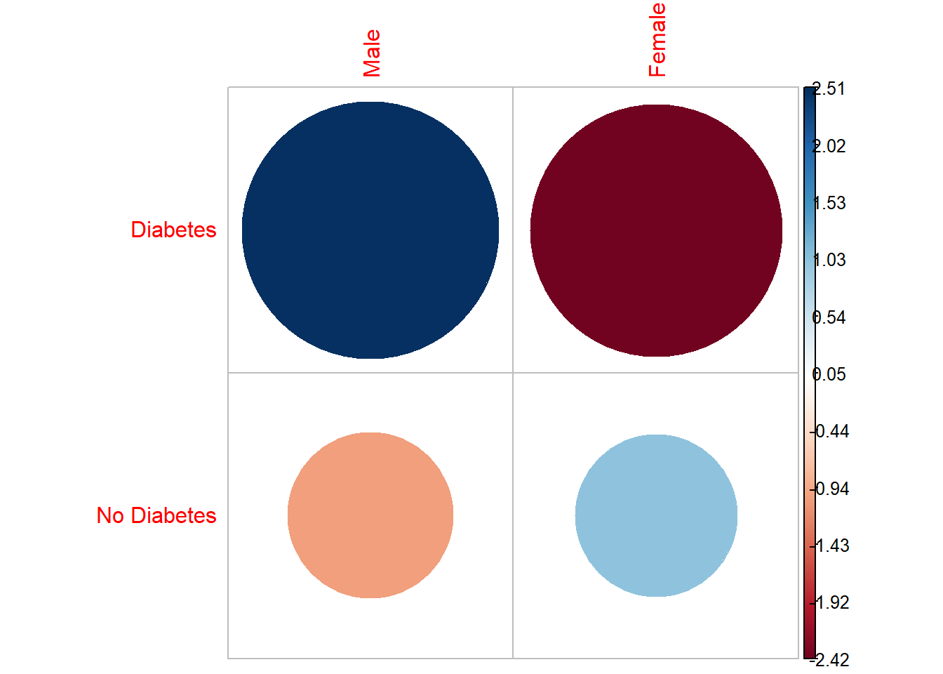
4.11.7 vcd
install_if_not('vcd')[1] "the package 'vcd' is already installed"vcd::assoc(table.sex_dm2, shade = TRUE, las=3)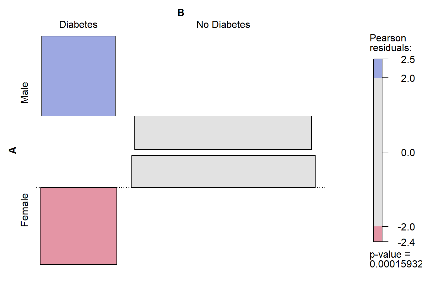
4.11.7.1 See also
4.12 T-Test
t.test(diab_pop$ridageyr ~ diab_pop$diq010)
Welch Two Sample t-test
data: diab_pop$ridageyr by diab_pop$diq010
t = 26.406, df = 1407.4, p-value < 2.2e-16
alternative hypothesis: true difference in means between group Diabetes and group No Diabetes is not equal to 0
95 percent confidence interval:
12.81607 14.87303
sample estimates:
mean in group Diabetes mean in group No Diabetes
61.33768 47.49313 library(ggplot2)
# Basic box plot
p <- ggplot(diab_pop, aes(x=diq010 , y=ridageyr)) +
geom_boxplot()
p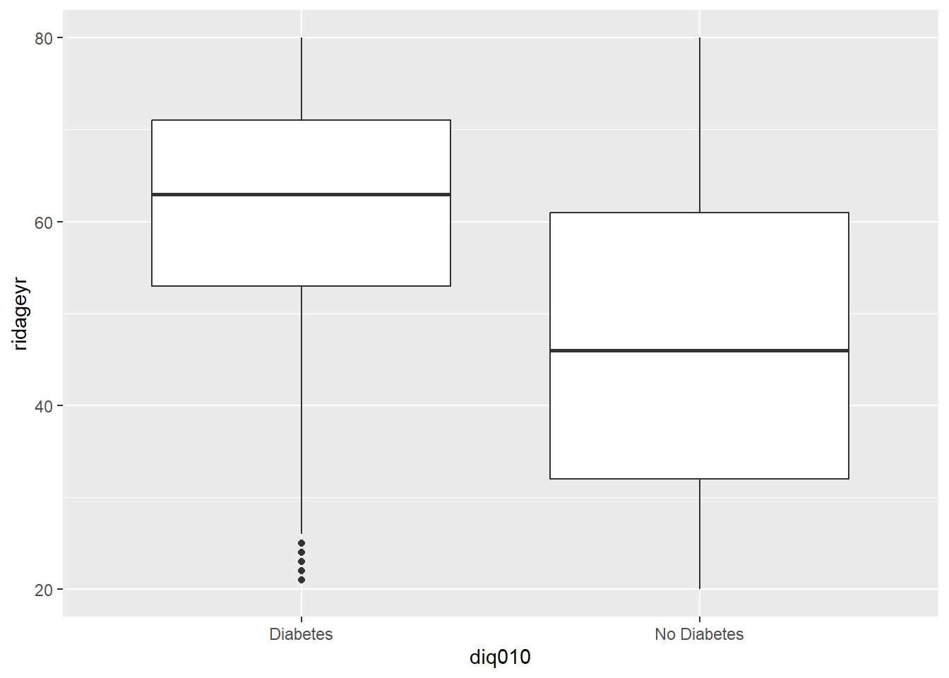
Welch Two Sample t-test
data: diab_pop.age.NoDM2 and diab_pop.age.DM2
t = -26.406, df = 1407.4, p-value < 2.2e-16
alternative hypothesis: true difference in means is not equal to 0
95 percent confidence interval:
-14.87303 -12.81607
sample estimates:
mean of x mean of y
47.49313 61.33768 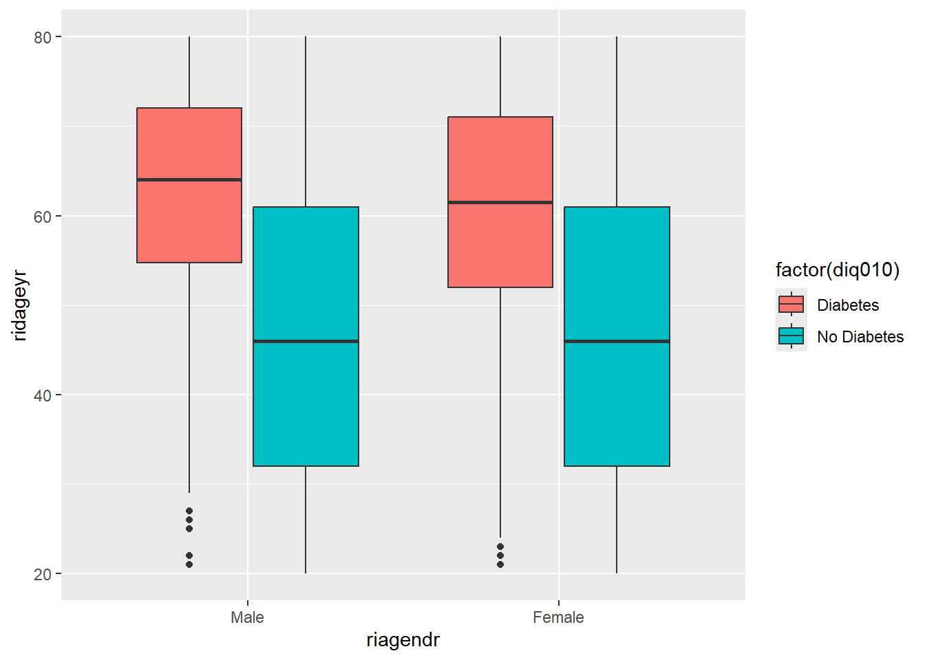
List of 10
$ statistic : Named num -26.4
..- attr(*, "names")= chr "t"
$ parameter : Named num 1407
..- attr(*, "names")= chr "df"
$ p.value : num 3.83e-125
$ conf.int : num [1:2] -14.9 -12.8
..- attr(*, "conf.level")= num 0.95
$ estimate : Named num [1:2] 47.5 61.3
..- attr(*, "names")= chr [1:2] "mean of x" "mean of y"
$ null.value : Named num 0
..- attr(*, "names")= chr "difference in means"
$ stderr : num 0.524
$ alternative: chr "two.sided"
$ method : chr "Welch Two Sample t-test"
$ data.name : chr "diab_pop.age.NoDM2 and diab_pop.age.DM2"
- attr(*, "class")= chr "htest"ttest_reults$p.value[1] 3.825137e-125broom::tidy(ttest_reults)# A tibble: 1 × 10
estimate estimate1 estimate2 statistic p.value parameter conf.low conf.high
<dbl> <dbl> <dbl> <dbl> <dbl> <dbl> <dbl> <dbl>
1 -13.8 47.5 61.3 -26.4 3.83e-125 1407. -14.9 -12.8
# ℹ 2 more variables: method <chr>, alternative <chr>broom::tidy(ttest_reults)$p.value[1] 3.825137e-125
4.13 ggplot2
ggplot(diab_pop, aes(bmxbmi, fill=diq010) ) +
geom_histogram(binwidth = 1) +
labs(title="BMI Distribution by Diabetes")Warning: Removed 313 rows containing non-finite outside the scale range
(`stat_bin()`).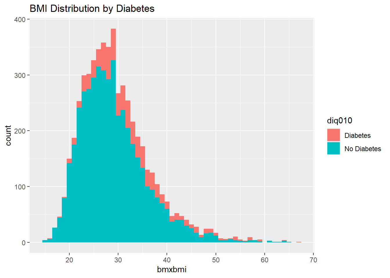
ggplot(diab_pop, aes(x=ridageyr, y=bmxbmi, shape=diq010, color=diq010)) +
geom_point() +
geom_smooth(method=lm , aes(fill=diq010)) +
labs(title="Scatter Plot of Age by BMI by Diabetes")`geom_smooth()` using formula = 'y ~ x'Warning: Removed 313 rows containing non-finite outside the scale range
(`stat_smooth()`).Warning: Removed 313 rows containing missing values or values outside the scale range
(`geom_point()`).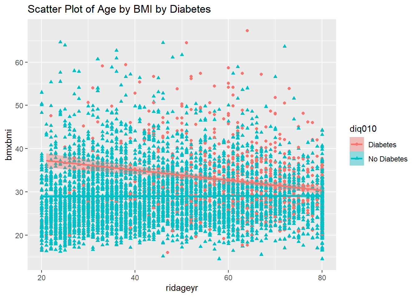
4.13.1 ggplot - Additional Resources
- ggplot cookbook : http://www.cookbook-r.com/Graphs/
- Top 50 ggplot Visualizations : http://r-statistics.co/Top50-Ggplot2-Visualizations-MasterList-R-Code.html
4.14 dplyr Revisited
Let’s look at some more complicated summary tables that we can produce
# A tibble: 12 × 12
# Groups: diq010, riagendr [4]
diq010 riagendr age_ntile ridageyr_min bmxbmi_min lbxglu_min ridageyr_mean
<fct> <fct> <int> <dbl> <dbl> <dbl> <dbl>
1 Diabetes Male 1 21 NA NA 31.5
2 Diabetes Male 2 39 NA NA 51.5
3 Diabetes Male 3 60 NA NA 69.9
4 Diabetes Female 1 21 NA NA 31.6
5 Diabetes Female 2 39 NA NA 50.2
6 Diabetes Female 3 60 NA NA 69.6
7 No Diabe… Male 1 20 NA NA 29.4
8 No Diabe… Male 2 39 NA NA 49.1
9 No Diabe… Male 3 59 NA NA 70.2
10 No Diabe… Female 1 20 NA NA 29.2
11 No Diabe… Female 2 39 NA NA 48.6
12 No Diabe… Female 3 59 NA NA 70.5
# ℹ 5 more variables: bmxbmi_mean <dbl>, lbxglu_mean <dbl>, ridageyr_max <dbl>,
# bmxbmi_max <dbl>, lbxglu_max <dbl># A tibble: 12 × 6
# Groups: diq010, riagendr [4]
diq010 riagendr age_ntile min mean max
<fct> <fct> <int> <dbl> <dbl> <dbl>
1 Diabetes Male 1 21 31.5 39
2 Diabetes Male 2 39 51.5 59
3 Diabetes Male 3 60 69.9 80
4 Diabetes Female 1 21 31.6 39
5 Diabetes Female 2 39 50.2 59
6 Diabetes Female 3 60 69.6 80
7 No Diabetes Male 1 20 29.4 39
8 No Diabetes Male 2 39 49.1 59
9 No Diabetes Male 3 59 70.2 80
10 No Diabetes Female 1 20 29.2 39
11 No Diabetes Female 2 39 48.6 59
12 No Diabetes Female 3 59 70.5 80We can also store our results of our dplyr query as a new dataframe:
# A tibble: 12 × 12
diq010 riagendr age_ntile ridageyr_min bmxbmi_min lbxglu_min ridageyr_mean
<fct> <fct> <int> <dbl> <dbl> <dbl> <dbl>
1 Diabetes Male 1 21 19.8 76 31.5
2 Diabetes Male 2 39 16 21 51.5
3 Diabetes Male 3 60 17.7 68 69.9
4 Diabetes Female 1 21 24 84 31.6
5 Diabetes Female 2 39 19.6 75 50.2
6 Diabetes Female 3 60 17.7 50 69.6
7 No Diabe… Male 1 20 16.2 70 29.4
8 No Diabe… Male 2 39 15.1 74 49.1
9 No Diabe… Male 3 59 16.4 64 70.2
10 No Diabe… Female 1 20 16.3 74 29.2
11 No Diabe… Female 2 39 14.5 77 48.6
12 No Diabe… Female 3 59 14.5 64 70.5
# ℹ 5 more variables: bmxbmi_mean <dbl>, lbxglu_mean <dbl>, ridageyr_max <dbl>,
# bmxbmi_max <dbl>, lbxglu_max <dbl>We can pass in user defined functions where they make sense:
# A tibble: 12 × 6
diq010 riagendr age_ntile ridageyr_SumNa bmxbmi_SumNa lbxglu_SumNa
<fct> <fct> <int> <int> <int> <int>
1 Diabetes Male 1 0 2 18
2 Diabetes Male 2 0 3 79
3 Diabetes Male 3 0 24 155
4 Diabetes Female 1 0 1 18
5 Diabetes Female 2 0 5 64
6 Diabetes Female 3 0 20 128
7 No Diabetes Male 1 0 57 531
8 No Diabetes Male 2 0 29 420
9 No Diabetes Male 3 0 49 360
10 No Diabetes Female 1 0 44 576
11 No Diabetes Female 2 0 43 515
12 No Diabetes Female 3 0 36 403We can join our two tables by the ridageyr,bmxbmi, and lbxglu values:
# A tibble: 12 × 15
diq010 riagendr age_ntile ridageyr_min bmxbmi_min lbxglu_min ridageyr_mean
<fct> <fct> <int> <dbl> <dbl> <dbl> <dbl>
1 Diabetes Male 1 21 19.8 76 31.5
2 Diabetes Male 2 39 16 21 51.5
3 Diabetes Male 3 60 17.7 68 69.9
4 Diabetes Female 1 21 24 84 31.6
5 Diabetes Female 2 39 19.6 75 50.2
6 Diabetes Female 3 60 17.7 50 69.6
7 No Diabe… Male 1 20 16.2 70 29.4
8 No Diabe… Male 2 39 15.1 74 49.1
9 No Diabe… Male 3 59 16.4 64 70.2
10 No Diabe… Female 1 20 16.3 74 29.2
11 No Diabe… Female 2 39 14.5 77 48.6
12 No Diabe… Female 3 59 14.5 64 70.5
# ℹ 8 more variables: bmxbmi_mean <dbl>, lbxglu_mean <dbl>, ridageyr_max <dbl>,
# bmxbmi_max <dbl>, lbxglu_max <dbl>, ridageyr_SumNa <int>,
# bmxbmi_SumNa <int>, lbxglu_SumNa <int>We can also get the same result with one query:
Let’s compare to make sure things are the same:
arsenal::comparedf(Table_Stats_3,Table_Stats_3a)Compare Object
Function Call:
arsenal::comparedf(x = Table_Stats_3, y = Table_Stats_3a)
Shared: 15 non-by variables and 12 observations.
Not shared: 0 variables and 0 observations.
Differences found in 0/15 variables compared.
0 variables compared have non-identical attributes.
4.15 The tidyverse
Even when we create a summary table things can be complicated, this result will have 3+(3*6) = 21 columns. In this section we will see even more of the data wrangling capabilities in the tidyverse
Table_Stats_3b <- diab_pop %>%
mutate(age_ntile = ntile(ridageyr,3)) %>%
group_by(diq010,riagendr,age_ntile) %>%
summarise_at(vars(ridageyr,bmxbmi,lbxglu), list(cnt =~ n() ,
min = ~ min(.,na.rm=TRUE),
mean= ~ mean(.,na.rm=TRUE),
sd = ~ sd(.,na.rm=TRUE),
max = ~ max(.,na.rm=TRUE),
SumNa =~ SumNa(.))
) %>%
ungroup()
colnames(Table_Stats_3b) [1] "diq010" "riagendr" "age_ntile" "ridageyr_cnt"
[5] "bmxbmi_cnt" "lbxglu_cnt" "ridageyr_min" "bmxbmi_min"
[9] "lbxglu_min" "ridageyr_mean" "bmxbmi_mean" "lbxglu_mean"
[13] "ridageyr_sd" "bmxbmi_sd" "lbxglu_sd" "ridageyr_max"
[17] "bmxbmi_max" "lbxglu_max" "ridageyr_SumNa" "bmxbmi_SumNa"
[21] "lbxglu_SumNa" ncol(Table_Stats_3b)[1] 21Table_Stats_3b# A tibble: 12 × 21
diq010 riagendr age_ntile ridageyr_cnt bmxbmi_cnt lbxglu_cnt ridageyr_min
<fct> <fct> <int> <int> <int> <int> <dbl>
1 Diabetes Male 1 25 25 25 21
2 Diabetes Male 2 136 136 136 39
3 Diabetes Male 3 295 295 295 60
4 Diabetes Female 1 33 33 33 21
5 Diabetes Female 2 124 124 124 39
6 Diabetes Female 3 231 231 231 60
7 No Diabet… Male 1 889 889 889 20
8 No Diabet… Male 2 750 750 750 39
9 No Diabet… Male 3 652 652 652 59
10 No Diabet… Female 1 960 960 960 20
11 No Diabet… Female 2 896 896 896 39
12 No Diabet… Female 3 728 728 728 59
# ℹ 14 more variables: bmxbmi_min <dbl>, lbxglu_min <dbl>, ridageyr_mean <dbl>,
# bmxbmi_mean <dbl>, lbxglu_mean <dbl>, ridageyr_sd <dbl>, bmxbmi_sd <dbl>,
# lbxglu_sd <dbl>, ridageyr_max <dbl>, bmxbmi_max <dbl>, lbxglu_max <dbl>,
# ridageyr_SumNa <int>, bmxbmi_SumNa <int>, lbxglu_SumNa <int>The gather command is used to “un-pivot” a dataframe, it makes a “wide” data-frame longer. Here I am gathering all columns except for diq010,riagendr,age_ntile, the column names will be placed in Feature_Type and the values will be placed in Value:
# A tibble: 216 × 5
diq010 riagendr age_ntile Feature_Type Value
<fct> <fct> <int> <chr> <dbl>
1 Diabetes Male 1 ridageyr_cnt 25
2 Diabetes Male 2 ridageyr_cnt 136
3 Diabetes Male 3 ridageyr_cnt 295
4 Diabetes Female 1 ridageyr_cnt 33
5 Diabetes Female 2 ridageyr_cnt 124
6 Diabetes Female 3 ridageyr_cnt 231
7 No Diabetes Male 1 ridageyr_cnt 889
8 No Diabetes Male 2 ridageyr_cnt 750
9 No Diabetes Male 3 ridageyr_cnt 652
10 No Diabetes Female 1 ridageyr_cnt 960
# ℹ 206 more rowsThe separate command can be used to separate a column into two columns using a delimiter. Here I am separating Feature_Type into Feature and Type:
# A tibble: 216 × 6
diq010 riagendr age_ntile Feature Type Value
<fct> <fct> <int> <chr> <chr> <dbl>
1 Diabetes Male 1 ridageyr cnt 25
2 Diabetes Male 2 ridageyr cnt 136
3 Diabetes Male 3 ridageyr cnt 295
4 Diabetes Female 1 ridageyr cnt 33
5 Diabetes Female 2 ridageyr cnt 124
6 Diabetes Female 3 ridageyr cnt 231
7 No Diabetes Male 1 ridageyr cnt 889
8 No Diabetes Male 2 ridageyr cnt 750
9 No Diabetes Male 3 ridageyr cnt 652
10 No Diabetes Female 1 ridageyr cnt 960
# ℹ 206 more rowsThe spread function is the opposite of gather, it is used to pivot a dataframe and makes data go from a “wide” to “long” format:
# A tibble: 36 × 10
diq010 riagendr age_ntile Feature cnt max mean min sd SumNa
<fct> <fct> <int> <chr> <dbl> <dbl> <dbl> <dbl> <dbl> <dbl>
1 Diabetes Male 1 bmxbmi 25 54 32.5 19.8 8.87 2
2 Diabetes Male 1 lbxglu 25 369 209. 76 120. 18
3 Diabetes Male 1 ridageyr 25 39 31.5 21 5.36 0
4 Diabetes Male 2 bmxbmi 136 57.4 32.6 16 8.12 3
5 Diabetes Male 2 lbxglu 136 454 176. 21 78.8 79
6 Diabetes Male 2 ridageyr 136 59 51.5 39 5.23 0
7 Diabetes Male 3 bmxbmi 295 54.2 30.7 17.7 6.22 24
8 Diabetes Male 3 lbxglu 295 479 163. 68 68.0 155
9 Diabetes Male 3 ridageyr 295 80 69.9 60 6.41 0
10 Diabetes Female 1 bmxbmi 33 59.4 36.6 24 9.07 1
# ℹ 26 more rowsWe can now add new columns that we might be interested in:
# A tibble: 36 × 11
diq010 riagendr age_ntile Feature cnt max mean min sd SumNa pct_NA
<fct> <fct> <int> <chr> <dbl> <dbl> <dbl> <dbl> <dbl> <dbl> <dbl>
1 Diabe… Male 1 bmxbmi 25 54 32.5 19.8 8.87 2 0.08
2 Diabe… Male 1 lbxglu 25 369 209. 76 120. 18 0.72
3 Diabe… Male 1 ridage… 25 39 31.5 21 5.36 0 0
4 Diabe… Male 2 bmxbmi 136 57.4 32.6 16 8.12 3 0.0221
5 Diabe… Male 2 lbxglu 136 454 176. 21 78.8 79 0.581
6 Diabe… Male 2 ridage… 136 59 51.5 39 5.23 0 0
7 Diabe… Male 3 bmxbmi 295 54.2 30.7 17.7 6.22 24 0.0814
8 Diabe… Male 3 lbxglu 295 479 163. 68 68.0 155 0.525
9 Diabe… Male 3 ridage… 295 80 69.9 60 6.41 0 0
10 Diabe… Female 1 bmxbmi 33 59.4 36.6 24 9.07 1 0.0303
# ℹ 26 more rowsWe can make R show us all the columns:
options(tibble.width = Inf)Table_Stats_7# A tibble: 36 × 11
diq010 riagendr age_ntile Feature cnt max mean min sd SumNa
<fct> <fct> <int> <chr> <dbl> <dbl> <dbl> <dbl> <dbl> <dbl>
1 Diabetes Male 1 bmxbmi 25 54 32.5 19.8 8.87 2
2 Diabetes Male 1 lbxglu 25 369 209. 76 120. 18
3 Diabetes Male 1 ridageyr 25 39 31.5 21 5.36 0
4 Diabetes Male 2 bmxbmi 136 57.4 32.6 16 8.12 3
5 Diabetes Male 2 lbxglu 136 454 176. 21 78.8 79
6 Diabetes Male 2 ridageyr 136 59 51.5 39 5.23 0
7 Diabetes Male 3 bmxbmi 295 54.2 30.7 17.7 6.22 24
8 Diabetes Male 3 lbxglu 295 479 163. 68 68.0 155
9 Diabetes Male 3 ridageyr 295 80 69.9 60 6.41 0
10 Diabetes Female 1 bmxbmi 33 59.4 36.6 24 9.07 1
pct_NA
<dbl>
1 0.08
2 0.72
3 0
4 0.0221
5 0.581
6 0
7 0.0814
8 0.525
9 0
10 0.0303
# ℹ 26 more rowsFinally we can sort to see the feature with the highest percentage of missing values is lbxglu among the lowest aged diabetic male population:
# A tibble: 36 × 11
diq010 riagendr age_ntile Feature cnt max mean min sd SumNa
<fct> <fct> <int> <chr> <dbl> <dbl> <dbl> <dbl> <dbl> <dbl>
1 Diabetes Male 1 lbxglu 25 369 209. 76 120. 18
2 No Diabetes Female 1 lbxglu 960 335 96.0 74 15.3 576
3 No Diabetes Male 1 lbxglu 889 322 101. 70 17.0 531
4 Diabetes Male 2 lbxglu 136 454 176. 21 78.8 79
5 No Diabetes Female 2 lbxglu 896 285 103. 77 20.5 515
6 No Diabetes Male 2 lbxglu 750 397 109. 74 27.5 420
7 Diabetes Female 3 lbxglu 231 461 160. 50 68.4 128
8 No Diabetes Female 3 lbxglu 728 309 109. 64 22.4 403
9 No Diabetes Male 3 lbxglu 652 234 108. 64 16.3 360
10 Diabetes Female 1 lbxglu 33 390 150. 84 79.9 18
pct_NA
<dbl>
1 0.72
2 0.6
3 0.597
4 0.581
5 0.575
6 0.56
7 0.554
8 0.554
9 0.552
10 0.545
# ℹ 26 more rowsAlthough we built the table one step at a time we can also string together our commands to achieve the same result:
── Attaching core tidyverse packages ──────────────────────── tidyverse 2.0.0 ──
✔ forcats 1.0.1 ✔ stringr 1.6.0
✔ lubridate 1.9.5 ✔ tibble 3.3.1
✔ purrr 1.2.2 ✔ tidyr 1.3.2
✔ readr 2.2.0
── Conflicts ────────────────────────────────────────── tidyverse_conflicts() ──
✖ dplyr::filter() masks mice::filter(), stats::filter()
✖ dplyr::lag() masks stats::lag()
ℹ Use the conflicted package (<http://conflicted.r-lib.org/>) to force all conflicts to become errorsTable_Stats_9 <- diab_pop %>%
mutate(age_ntile = ntile(ridageyr,3)) %>%
group_by(diq010,riagendr,age_ntile) %>%
summarise_at(vars(ridageyr,bmxbmi,lbxglu), list(cnt =~ n() ,
min = ~ min(.,na.rm=TRUE),
mean= ~ mean(.,na.rm=TRUE),
sd = ~ sd(.,na.rm=TRUE),
max = ~ max(.,na.rm=TRUE),
SumNa =~ SumNa(.))
) %>%
ungroup() %>%
gather(-diq010,-riagendr,-age_ntile, key="Feature_Type", value="Value") %>%
separate(Feature_Type,into=c('Feature','Type')) %>%
spread(key='Type',value='Value') %>%
mutate(pct_NA = SumNa/cnt) %>%
arrange(desc(pct_NA))
Table_Stats_9# A tibble: 36 × 11
diq010 riagendr age_ntile Feature cnt max mean min sd SumNa
<fct> <fct> <int> <chr> <dbl> <dbl> <dbl> <dbl> <dbl> <dbl>
1 Diabetes Male 1 lbxglu 25 369 209. 76 120. 18
2 No Diabetes Female 1 lbxglu 960 335 96.0 74 15.3 576
3 No Diabetes Male 1 lbxglu 889 322 101. 70 17.0 531
4 Diabetes Male 2 lbxglu 136 454 176. 21 78.8 79
5 No Diabetes Female 2 lbxglu 896 285 103. 77 20.5 515
6 No Diabetes Male 2 lbxglu 750 397 109. 74 27.5 420
7 Diabetes Female 3 lbxglu 231 461 160. 50 68.4 128
8 No Diabetes Female 3 lbxglu 728 309 109. 64 22.4 403
9 No Diabetes Male 3 lbxglu 652 234 108. 64 16.3 360
10 Diabetes Female 1 lbxglu 33 390 150. 84 79.9 18
pct_NA
<dbl>
1 0.72
2 0.6
3 0.597
4 0.581
5 0.575
6 0.56
7 0.554
8 0.554
9 0.552
10 0.545
# ℹ 26 more rowsarsenal::comparedf(Table_Stats_8,Table_Stats_9)Compare Object
Function Call:
arsenal::comparedf(x = Table_Stats_8, y = Table_Stats_9)
Shared: 11 non-by variables and 36 observations.
Not shared: 0 variables and 0 observations.
Differences found in 0/11 variables compared.
0 variables compared have non-identical attributes.4.15.1 See also
-
tidyverse: https://www.tidyverse.org/ -
Rfor Data Science: https://r4ds.had.co.nz/ - Modern
Rwith thetidyverse: https://b-rodrigues.github.io/modern_R/
4.16 One Hot Encoding
Often categorical variables are encoded into binary 0 or 1 flags of new features.
`summarise()` has regrouped the output.
ℹ Summaries were computed grouped by diq010 and riagendr.
ℹ Output is grouped by diq010.
ℹ Use `summarise(.groups = "drop_last")` to silence this message.
ℹ Use `summarise(.by = c(diq010, riagendr))` for per-operation grouping
(`?dplyr::dplyr_by`) instead.# A tibble: 4 × 3
# Groups: diq010 [2]
diq010 riagendr cnt
<fct> <fct> <int>
1 Diabetes Male 456
2 Diabetes Female 388
3 No Diabetes Male 2291
4 No Diabetes Female 2584Rows: 5,719
Columns: 12
$ seqn <dbl> 83732, 83733, 83734, 83735, 83736, 83737, 83741, 83742, 83744…
$ riagendr <fct> Male, Male, Male, Female, Female, Female, Male, Female, Male,…
$ ridageyr <dbl> 62, 53, 78, 56, 42, 72, 22, 32, 56, 46, 45, 30, 67, 67, 57, 8…
$ ridreth1 <fct> Non-Hispanic White, Non-Hispanic White, Non-Hispanic White, N…
$ dmdeduc2 <fct> College grad or above, High school graduate/GED, High school …
$ dmdmartl <fct> Married, Divorced, Married, Living with partner, Divorced, Se…
$ indhhin2 <fct> "$65,000-$74,999", "$15,000-$19,999", "$20,000-$24,999", "$65…
$ bmxbmi <dbl> 27.8, 30.8, 28.8, 42.4, 20.3, 28.6, 28.0, 28.2, 33.6, 27.6, 2…
$ diq010 <fct> Diabetes, No Diabetes, Diabetes, No Diabetes, No Diabetes, No…
$ lbxglu <dbl> NA, 101, 84, NA, 84, 107, 95, NA, NA, NA, 84, NA, 130, 284, 3…
$ SexMale <dbl> 1, 1, 1, 0, 0, 0, 1, 0, 1, 1, 1, 0, 0, 1, 0, 1, 0, 0, 0, 1, 0…
$ DM2 <dbl> 1, 0, 1, 0, 0, 0, 0, 0, 1, 0, 0, 0, 0, 1, 1, 0, 0, 0, 0, 0, 0…# A tibble: 2 × 2
DM2 cnt
<dbl> <dbl>
1 0 2291
2 1 456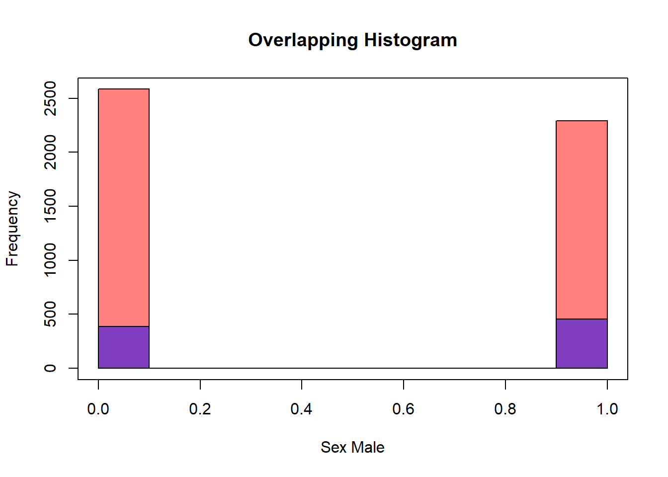
Of course encoding each categorical variable can take time so we can use the dummyVars function in the caret package:
Attaching package: 'caret'The following object is masked from 'package:purrr':
liftList of 9
$ call : language dummyVars.default(formula = " ~ .", data = diab_pop)
$ form :Class 'formula' language ~.
.. ..- attr(*, ".Environment")=<environment: 0x000001da1221c2e0>
$ vars : chr [1:10] "seqn" "riagendr" "ridageyr" "ridreth1" ...
$ facVars : chr [1:6] "riagendr" "ridreth1" "dmdeduc2" "dmdmartl" ...
$ lvls :List of 6
..$ riagendr: chr [1:2] "Male" "Female"
..$ ridreth1: chr [1:5] "MexicanAmerican" "Other Hispanic" "Non-Hispanic White" "Non-Hispanic Black" ...
..$ dmdeduc2: chr [1:5] "Less than 9th grade" "Grades 9-11th" "High school graduate/GED" "Some college or AA degrees" ...
..$ dmdmartl: chr [1:6] "Married" "Widowed" "Divorced" "Separated" ...
..$ indhhin2: chr [1:14] "$0-$4,999" "$5,000-$9,999" "$10,000-$14,999" "$15,000-$19,999" ...
..$ diq010 : chr [1:2] "Diabetes" "No Diabetes"
$ sep : chr "."
$ terms :Classes 'terms', 'formula' language ~seqn + riagendr + ridageyr + ridreth1 + dmdeduc2 + dmdmartl + indhhin2 + bmxbmi + diq010 + lbxglu
.. ..- attr(*, "variables")= language list(seqn, riagendr, ridageyr, ridreth1, dmdeduc2, dmdmartl, indhhin2, bmxbmi, diq010, lbxglu)
.. ..- attr(*, "factors")= int [1:10, 1:10] 1 0 0 0 0 0 0 0 0 0 ...
.. .. ..- attr(*, "dimnames")=List of 2
.. .. .. ..$ : chr [1:10] "seqn" "riagendr" "ridageyr" "ridreth1" ...
.. .. .. ..$ : chr [1:10] "seqn" "riagendr" "ridageyr" "ridreth1" ...
.. ..- attr(*, "term.labels")= chr [1:10] "seqn" "riagendr" "ridageyr" "ridreth1" ...
.. ..- attr(*, "order")= int [1:10] 1 1 1 1 1 1 1 1 1 1
.. ..- attr(*, "intercept")= int 1
.. ..- attr(*, "response")= int 0
.. ..- attr(*, ".Environment")=<environment: 0x000001da1221c2e0>
.. ..- attr(*, "predvars")= language list(seqn, riagendr, ridageyr, ridreth1, dmdeduc2, dmdmartl, indhhin2, bmxbmi, diq010, lbxglu)
.. ..- attr(*, "dataClasses")= Named chr [1:10] "numeric" "factor" "numeric" "factor" ...
.. .. ..- attr(*, "names")= chr [1:10] "seqn" "riagendr" "ridageyr" "ridreth1" ...
$ levelsOnly: logi FALSE
$ fullRank : logi FALSE
- attr(*, "class")= chr "dummyVars" num [1:5719, 1:38] 83732 83733 83734 83735 83736 ...
- attr(*, "dimnames")=List of 2
..$ : chr [1:5719] "1" "2" "3" "4" ...
..$ : chr [1:38] "seqn" "riagendr.Male" "riagendr.Female" "ridageyr" ...tibble [5,719 × 38] (S3: tbl_df/tbl/data.frame)
$ seqn : num [1:5719] 83732 83733 83734 83735 83736 ...
$ riagendr.Male : num [1:5719] 1 1 1 0 0 0 1 0 1 1 ...
$ riagendr.Female : num [1:5719] 0 0 0 1 1 1 0 1 0 0 ...
$ ridageyr : num [1:5719] 62 53 78 56 42 72 22 32 56 46 ...
$ ridreth1.MexicanAmerican : num [1:5719] 0 0 0 0 0 1 0 1 0 0 ...
$ ridreth1.Other Hispanic : num [1:5719] 0 0 0 0 0 0 0 0 0 0 ...
$ ridreth1.Non-Hispanic White : num [1:5719] 1 1 1 1 0 0 0 0 0 1 ...
$ ridreth1.Non-Hispanic Black : num [1:5719] 0 0 0 0 1 0 1 0 1 0 ...
$ ridreth1.Other : num [1:5719] 0 0 0 0 0 0 0 0 0 0 ...
$ dmdeduc2.Less than 9th grade : num [1:5719] 0 0 0 0 0 0 0 0 0 0 ...
$ dmdeduc2.Grades 9-11th : num [1:5719] 0 0 0 0 0 1 0 0 0 0 ...
$ dmdeduc2.High school graduate/GED : num [1:5719] 0 1 1 0 0 0 0 0 1 0 ...
$ dmdeduc2.Some college or AA degrees: num [1:5719] 0 0 0 0 1 0 1 1 0 0 ...
$ dmdeduc2.College grad or above : num [1:5719] 1 0 0 1 0 0 0 0 0 1 ...
$ dmdmartl.Married : num [1:5719] 1 0 1 0 0 0 0 1 0 0 ...
$ dmdmartl.Widowed : num [1:5719] 0 0 0 0 0 0 0 0 0 0 ...
$ dmdmartl.Divorced : num [1:5719] 0 1 0 0 1 0 0 0 1 0 ...
$ dmdmartl.Separated : num [1:5719] 0 0 0 0 0 1 0 0 0 0 ...
$ dmdmartl.Never married : num [1:5719] 0 0 0 0 0 0 1 0 0 0 ...
$ dmdmartl.Living with partner : num [1:5719] 0 0 0 1 0 0 0 0 0 1 ...
$ indhhin2.$0-$4,999 : num [1:5719] 0 0 0 0 NA 0 NA 0 0 0 ...
$ indhhin2.$5,000-$9,999 : num [1:5719] 0 0 0 0 NA 0 NA 0 0 0 ...
$ indhhin2.$10,000-$14,999 : num [1:5719] 0 0 0 0 NA 0 NA 0 1 1 ...
$ indhhin2.$15,000-$19,999 : num [1:5719] 0 1 0 0 NA 0 NA 0 0 0 ...
$ indhhin2.$20,000-$24,999 : num [1:5719] 0 0 1 0 NA 0 NA 0 0 0 ...
$ indhhin2.$25,000-$34,999 : num [1:5719] 0 0 0 0 NA 0 NA 1 0 0 ...
$ indhhin2.$35,000-$44,999 : num [1:5719] 0 0 0 0 NA 0 NA 0 0 0 ...
$ indhhin2.$45,000-$54,999 : num [1:5719] 0 0 0 0 NA 0 NA 0 0 0 ...
$ indhhin2.$55,000-$64,999 : num [1:5719] 0 0 0 0 NA 0 NA 0 0 0 ...
$ indhhin2.$65,000-$74,999 : num [1:5719] 1 0 0 1 NA 0 NA 0 0 0 ...
$ indhhin2.20,000+ : num [1:5719] 0 0 0 0 NA 0 NA 0 0 0 ...
$ indhhin2.less than $20,000 : num [1:5719] 0 0 0 0 NA 0 NA 0 0 0 ...
$ indhhin2.$75,000-$99,999 : num [1:5719] 0 0 0 0 NA 1 NA 0 0 0 ...
$ indhhin2.$100,000+ : num [1:5719] 0 0 0 0 NA 0 NA 0 0 0 ...
$ bmxbmi : num [1:5719] 27.8 30.8 28.8 42.4 20.3 28.6 28 28.2 33.6 27.6 ...
$ diq010.Diabetes : num [1:5719] 1 0 1 0 0 0 0 0 1 0 ...
$ diq010.No Diabetes : num [1:5719] 0 1 0 1 1 1 1 1 0 1 ...
$ lbxglu : num [1:5719] NA 101 84 NA 84 107 95 NA NA NA ...
In our last example we left a space in the column name dmdmartl.Never married here is one way to remove it:
Rows: 5,719
Columns: 10
$ seqn     <dbl> 83732, 83733, 83734, 83735, 83736, 83737, 83741, 83742, 83744…
$ riagendr <fct> Male, Male, Male, Female, Female, Female, Male, Female, Male,…
$ ridageyr <dbl> 62, 53, 78, 56, 42, 72, 22, 32, 56, 46, 45, 30, 67, 67, 57, 8…
$ ridreth1 <fct> Non-Hispanic White, Non-Hispanic White, Non-Hispanic White, N…
$ dmdeduc2 <fct> College grad or above, High school graduate/GED, High school …
$ dmdmartl <chr> "Married", "Divorced", "Married", "Living_with partner", "Div…
$ indhhin2 <fct> "$65,000-$74,999", "$15,000-$19,999", "$20,000-$24,999", "$65…
$ bmxbmi   <dbl> 27.8, 30.8, 28.8, 42.4, 20.3, 28.6, 28.0, 28.2, 33.6, 27.6, 2…
$ diq010   <fct> Diabetes, No Diabetes, Diabetes, No Diabetes, No Diabetes, No…
$ lbxglu   <dbl> NA, 101, 84, NA, 84, 107, 95, NA, NA, NA, 84, NA, 130, 284, 3…
The stringr::str_replace function only replaced the first whitespace so that “Living with partner” is now “Living_with partner”. We can use str_replace_all instead to get “Living_with_partner”.
Rows: 5,719
Columns: 10
$ seqn     <dbl> 83732, 83733, 83734, 83735, 83736, 83737, 83741, 83742, 83744…
$ riagendr <fct> Male, Male, Male, Female, Female, Female, Male, Female, Male,…
$ ridageyr <dbl> 62, 53, 78, 56, 42, 72, 22, 32, 56, 46, 45, 30, 67, 67, 57, 8…
$ ridreth1 <fct> Non-Hispanic White, Non-Hispanic White, Non-Hispanic White, N…
$ dmdeduc2 <fct> College grad or above, High school graduate/GED, High school …
$ dmdmartl <fct> Married, Divorced, Married, Living_with_partner, Divorced, Se…
$ indhhin2 <fct> "$65,000-$74,999", "$15,000-$19,999", "$20,000-$24,999", "$65…
$ bmxbmi   <dbl> 27.8, 30.8, 28.8, 42.4, 20.3, 28.6, 28.0, 28.2, 33.6, 27.6, 2…
$ diq010   <fct> Diabetes, No Diabetes, Diabetes, No Diabetes, No Diabetes, No…
$ lbxglu   <dbl> NA, 101, 84, NA, 84, 107, 95, NA, NA, NA, 84, NA, 130, 284, 3…
diab_pop_f1 <- diab_pop %>%
mutate(dmdmartl = str_replace_all(dmdmartl," ","_")) %>%
mutate(dmdmartl = as.factor(dmdmartl)) %>%
mutate(ridreth1 = str_replace_all(ridreth1," ","_")) %>%
mutate(ridreth1 = as.factor(ridreth1)) %>%
mutate(diq010 = str_replace_all(ridreth1," ","_")) %>%
mutate(diq010 = as.factor(diq010)) %>%
mutate(dmdeduc2 = str_replace_all(dmdeduc2," ","_") ) %>%
mutate(dmdeduc2 = as.factor(dmdeduc2)) %>%
mutate(indhhin2 = str_replace_all(indhhin2," ","_") ) %>%
mutate(indhhin2 = as.factor(indhhin2))
caret.dummyVars.diab_pop_f1 <- dummyVars(" ~ .", data = diab_pop_f1)
predict_dummyVars_diab_pop <- predict(caret.dummyVars.diab_pop_f1, newdata = diab_pop_f1)
encode.diab_pop_f1 <- as_tibble(predict_dummyVars_diab_pop)
glimpse(encode.diab_pop_f1)Rows: 5,719
Columns: 39
$ seqn <dbl> 83732, 83733, 83734, 83735, 83736,…
$ riagendr.Male <dbl> 1, 1, 1, 0, 0, 0, 1, 0, 1, 1, 1, 0…
$ riagendr.Female <dbl> 0, 0, 0, 1, 1, 1, 0, 1, 0, 0, 0, 1…
$ ridageyr <dbl> 62, 53, 78, 56, 42, 72, 22, 32, 56…
$ ridreth1.MexicanAmerican <dbl> 0, 0, 0, 0, 0, 1, 0, 1, 0, 0, 0, 0…
$ `ridreth1.Non-Hispanic_Black` <dbl> 0, 0, 0, 0, 1, 0, 1, 0, 1, 0, 0, 0…
$ `ridreth1.Non-Hispanic_White` <dbl> 1, 1, 1, 1, 0, 0, 0, 0, 0, 1, 0, 0…
$ ridreth1.Other <dbl> 0, 0, 0, 0, 0, 0, 0, 0, 0, 0, 1, 0…
$ ridreth1.Other_Hispanic <dbl> 0, 0, 0, 0, 0, 0, 0, 0, 0, 0, 0, 1…
$ dmdeduc2.College_grad_or_above <dbl> 1, 0, 0, 1, 0, 0, 0, 0, 0, 1, 0, 0…
$ `dmdeduc2.Grades_9-11th` <dbl> 0, 0, 0, 0, 0, 1, 0, 0, 0, 0, 1, 0…
$ `dmdeduc2.High_school_graduate/GED` <dbl> 0, 1, 1, 0, 0, 0, 0, 0, 1, 0, 0, 0…
$ dmdeduc2.Less_than_9th_grade <dbl> 0, 0, 0, 0, 0, 0, 0, 0, 0, 0, 0, 0…
$ dmdeduc2.Some_college_or_AA_degrees <dbl> 0, 0, 0, 0, 1, 0, 1, 1, 0, 0, 0, 1…
$ dmdmartl.Divorced <dbl> 0, 1, 0, 0, 1, 0, 0, 0, 1, 0, 0, 0…
$ dmdmartl.Living_with_partner <dbl> 0, 0, 0, 1, 0, 0, 0, 0, 0, 1, 0, 1…
$ dmdmartl.Married <dbl> 1, 0, 1, 0, 0, 0, 0, 1, 0, 0, 0, 0…
$ dmdmartl.Never_married <dbl> 0, 0, 0, 0, 0, 0, 1, 0, 0, 0, 1, 0…
$ dmdmartl.Separated <dbl> 0, 0, 0, 0, 0, 1, 0, 0, 0, 0, 0, 0…
$ dmdmartl.Widowed <dbl> 0, 0, 0, 0, 0, 0, 0, 0, 0, 0, 0, 0…
$ `indhhin2.$0-$4,999` <dbl> 0, 0, 0, 0, NA, 0, NA, 0, 0, 0, 0,…
$ `indhhin2.$10,000-$14,999` <dbl> 0, 0, 0, 0, NA, 0, NA, 0, 1, 1, 0,…
$ `indhhin2.$100,000+` <dbl> 0, 0, 0, 0, NA, 0, NA, 0, 0, 0, 0,…
$ `indhhin2.$15,000-$19,999` <dbl> 0, 1, 0, 0, NA, 0, NA, 0, 0, 0, 0,…
$ `indhhin2.$20,000-$24,999` <dbl> 0, 0, 1, 0, NA, 0, NA, 0, 0, 0, 0,…
$ `indhhin2.$25,000-$34,999` <dbl> 0, 0, 0, 0, NA, 0, NA, 1, 0, 0, 0,…
$ `indhhin2.$45,000-$54,999` <dbl> 0, 0, 0, 0, NA, 0, NA, 0, 0, 0, 0,…
$ `indhhin2.$5,000-$9,999` <dbl> 0, 0, 0, 0, NA, 0, NA, 0, 0, 0, 0,…
$ `indhhin2.$65,000-$74,999` <dbl> 1, 0, 0, 1, NA, 0, NA, 0, 0, 0, 1,…
$ `indhhin2.$75,000-$99,999` <dbl> 0, 0, 0, 0, NA, 1, NA, 0, 0, 0, 0,…
$ `indhhin2.20,000+` <dbl> 0, 0, 0, 0, NA, 0, NA, 0, 0, 0, 0,…
$ `indhhin2.less_than_$20,000` <dbl> 0, 0, 0, 0, NA, 0, NA, 0, 0, 0, 0,…
$ bmxbmi <dbl> 27.8, 30.8, 28.8, 42.4, 20.3, 28.6…
$ diq010.MexicanAmerican <dbl> 0, 0, 0, 0, 0, 1, 0, 1, 0, 0, 0, 0…
$ `diq010.Non-Hispanic_Black` <dbl> 0, 0, 0, 0, 1, 0, 1, 0, 1, 0, 0, 0…
$ `diq010.Non-Hispanic_White` <dbl> 1, 1, 1, 1, 0, 0, 0, 0, 0, 1, 0, 0…
$ diq010.Other <dbl> 0, 0, 0, 0, 0, 0, 0, 0, 0, 0, 1, 0…
$ diq010.Other_Hispanic <dbl> 0, 0, 0, 0, 0, 0, 0, 0, 0, 0, 0, 1…
$ lbxglu <dbl> NA, 101, 84, NA, 84, 107, 95, NA, …Notice that we are applying the same functions to the columns, so another way to solve this issue might be with a function:
Then we can apply our function itteratively:
result1 <- my_replace_all_factor_function(diab_pop,dmdmartl)
result2 <- my_replace_all_factor_function(result1,ridreth1)
result3 <- my_replace_all_factor_function(result2,diq010)
result4 <- my_replace_all_factor_function(result3,dmdeduc2)
result5 <- my_replace_all_factor_function(result4,indhhin2)

arsenal::comparedf(diab_pop_f1 , result5)
Compare Object
Function Call:
arsenal::comparedf(x = diab_pop_f1, y = result5)
Shared: 10 non-by variables and 5719 observations.
Not shared: 0 variables and 0 observations.
Differences found in 1/10 variables compared.
1 variables compared have non-identical attributes.Here’s another way to apply our function:
Rows: 5,719
Columns: 10
$ seqn     <dbl> 83732, 83733, 83734, 83735, 83736, 83737, 83741, 83742, 83744…
$ riagendr <fct> Male, Male, Male, Female, Female, Female, Male, Female, Male,…
$ ridageyr <dbl> 62, 53, 78, 56, 42, 72, 22, 32, 56, 46, 45, 30, 67, 67, 57, 8…
$ ridreth1 <fct> Non-Hispanic_White, Non-Hispanic_White, Non-Hispanic_White, N…
$ dmdeduc2 <fct> College_grad_or_above, High_school_graduate/GED, High_school_…
$ dmdmartl <fct> Married, Divorced, Married, Living_with_partner, Divorced, Se…
$ indhhin2 <fct> "$65,000-$74,999", "$15,000-$19,999", "$20,000-$24,999", "$65…
$ bmxbmi   <dbl> 27.8, 30.8, 28.8, 42.4, 20.3, 28.6, 28.0, 28.2, 33.6, 27.6, 2…
$ diq010   <fct> Diabetes, No_Diabetes, Diabetes, No_Diabetes, No_Diabetes, No…
$ lbxglu <dbl> NA, 101, 84, NA, 84, 107, 95, NA, NA, NA, 84, NA, 130, 284, 3…arsenal::comparedf(result5 , result_f)Compare Object
Function Call:
arsenal::comparedf(x = result5, y = result_f)
Shared: 10 non-by variables and 5719 observations.
Not shared: 0 variables and 0 observations.
Differences found in 0/10 variables compared.
0 variables compared have non-identical attributes.4.16.1 addition resources: programming with dplyr
- programming with
dplyrvignette: https://cran.r-project.org/web/packages/dplyr/vignettes/programming.html
4.17 ks-test
Warning in ks.test.default(diab_pop.NoDM2.age, diab_pop.DM2.age): p-value will
be approximate in the presence of ties
[1] 1.334401e-92Now let’s create a table of some ks-tests. We can write a function to assist us:
ks_wrapper <- function(df, factor, factor_level,  continuous_feature){
  F <- NULL

  factor <- enquo(factor)

  data.local <- df %>%
    select(!! factor, continuous_feature)

  X <- data.local %>%
    filter(!! factor == factor_level)

  Y <- data.local %>%
    filter(!(!! factor == factor_level))

  F$x <- X[,continuous_feature]
  F$y <- Y[,continuous_feature]

  ks_test_stat_T <- ks.test(F$x,F$y)
  ks_test_stat <- ks_test_stat_T$p.value

  result_row <- tibble::enframe(ks_test_stat)

  result_row <- result_row %>%
    mutate(Feature = continuous_feature)

  return(result_row)
  }
A single call to the function will give us a table with the p-value of the ks-test:
Warning: Using an external vector in selections was deprecated in tidyselect 1.1.0.
ℹ Please use `all_of()` or `any_of()` instead.
  # Was:
  data %>% select(continuous_feature)

  # Now:
  data %>% select(all_of(continuous_feature))

See <https://tidyselect.r-lib.org/reference/faq-external-vector.html>.
Warning in ks.test.default(F$x, F$y): p-value will be approximate in the
presence of ties# A tibble: 1 × 3
name value Feature
<int> <dbl> <chr>
1 1 1.33e-92 ridageyrWe can iterate our function over other columns and use purrr::map_dfr to make a single table:
Warning in ks.test.default(F$x, F$y): p-value will be approximate in the
presence of ties
Warning in ks.test.default(F$x, F$y): p-value will be approximate in the
presence of ties
Warning in ks.test.default(F$x, F$y): p-value will be approximate in the
presence of tiesks_test_results_table# A tibble: 3 × 3
name value Feature
<int> <dbl> <chr>
1 1 1.33e- 92 ridageyr
2 1 1.00e- 27 bmxbmi
3 1 3.52e-111 lbxglu # A tibble: 3 × 3
name ks_test_p_value Feature
<int> <dbl> <chr>
1 1 1.33e- 92 ridageyr
2 1 1.00e- 27 bmxbmi
3 1 3.52e-111 lbxglu We can add to the table, by finding some related values to showcase along:
means.diab_pop_f2 <- diab_pop_f2 %>%
  group_by(DM2_num) %>%
  summarise_at(vars(c('ridageyr','bmxbmi','lbxglu')), list(~mean(.,na.rm = TRUE),~sd(.,na.rm = TRUE))) %>%
  gather(-DM2_num, key="Feature_Type", value="Value") %>%
  separate(Feature_Type, into= c('Feature','Type'), sep='_') %>%
  mutate(DM2_stats_char = ifelse(DM2_num == 1,"Diabetes","No_Diabetes")) %>%
  mutate(DM2_stats_char_Type = paste0(DM2_stats_char,"_",Type)) %>%
  select(-DM2_num,-Type,-DM2_stats_char) %>%
  select(Feature, DM2_stats_char_Type, Value) %>%
  spread(key='DM2_stats_char_Type', value = 'Value')

means.diab_pop_f2
# A tibble: 3 × 5
Feature Diabetes_mean Diabetes_sd No_Diabetes_mean No_Diabetes_sd
<chr> <dbl> <dbl> <dbl> <dbl>
1 bmxbmi 32.6 7.73 29.0 6.82
2 lbxglu 166. 73.5 104. 20.7
3 ridageyr 61.3 13.3 47.5 17.6 Finally we can join our tables together:
Joining with `by = join_by(Feature)`ks_table_1# A tibble: 3 × 6
Feature Diabetes_mean Diabetes_sd ks_test_p_value No_Diabetes_mean
<chr> <dbl> <dbl> <dbl> <dbl>
1 ridageyr 61.3 13.3 1.33e- 92 47.5
2 bmxbmi 32.6 7.73 1.00e- 27 29.0
3 lbxglu 166. 73.5 3.52e-111 104.
No_Diabetes_sd
<dbl>
1 17.6
2 6.82
3 20.7 We can also use R to make the table more presentable:
install_if_not('kableExtra')[1] "the package 'kableExtra' is already installed"
Attaching package: 'kableExtra'The following object is masked from 'package:dplyr':
group_rowsks_table_style <- kable(ks_table_1) %>%
kable_styling("striped") %>%
add_header_above(c(" " = 1, "Diabetes" = 2, "ks-test pvalue" = 1, "Non Diabetes" = 2))
ks_table_style| Feature | Diabetes_mean | Diabetes_sd | ks_test_p_value | No_Diabetes_mean | No_Diabetes_sd |
|---|---|---|---|---|---|
| ridageyr | 61.33768 | 13.347476 | 0 | 47.49313 | 17.635870 |
| bmxbmi | 32.59632 | 7.733781 | 0 | 29.01988 | 6.823482 |
| lbxglu | 165.98953 | 73.475333 | 0 | 103.94155 | 20.720142 |
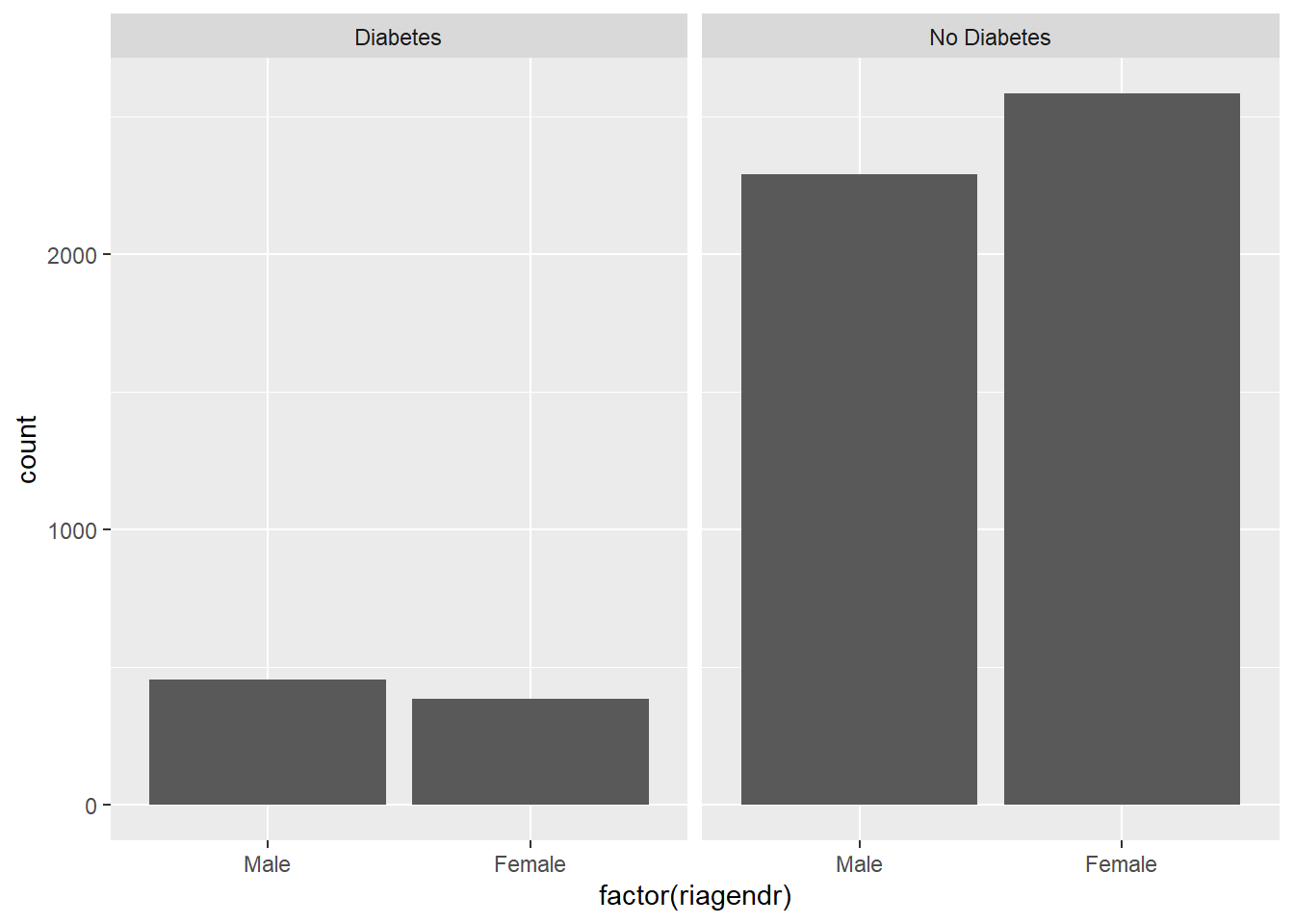
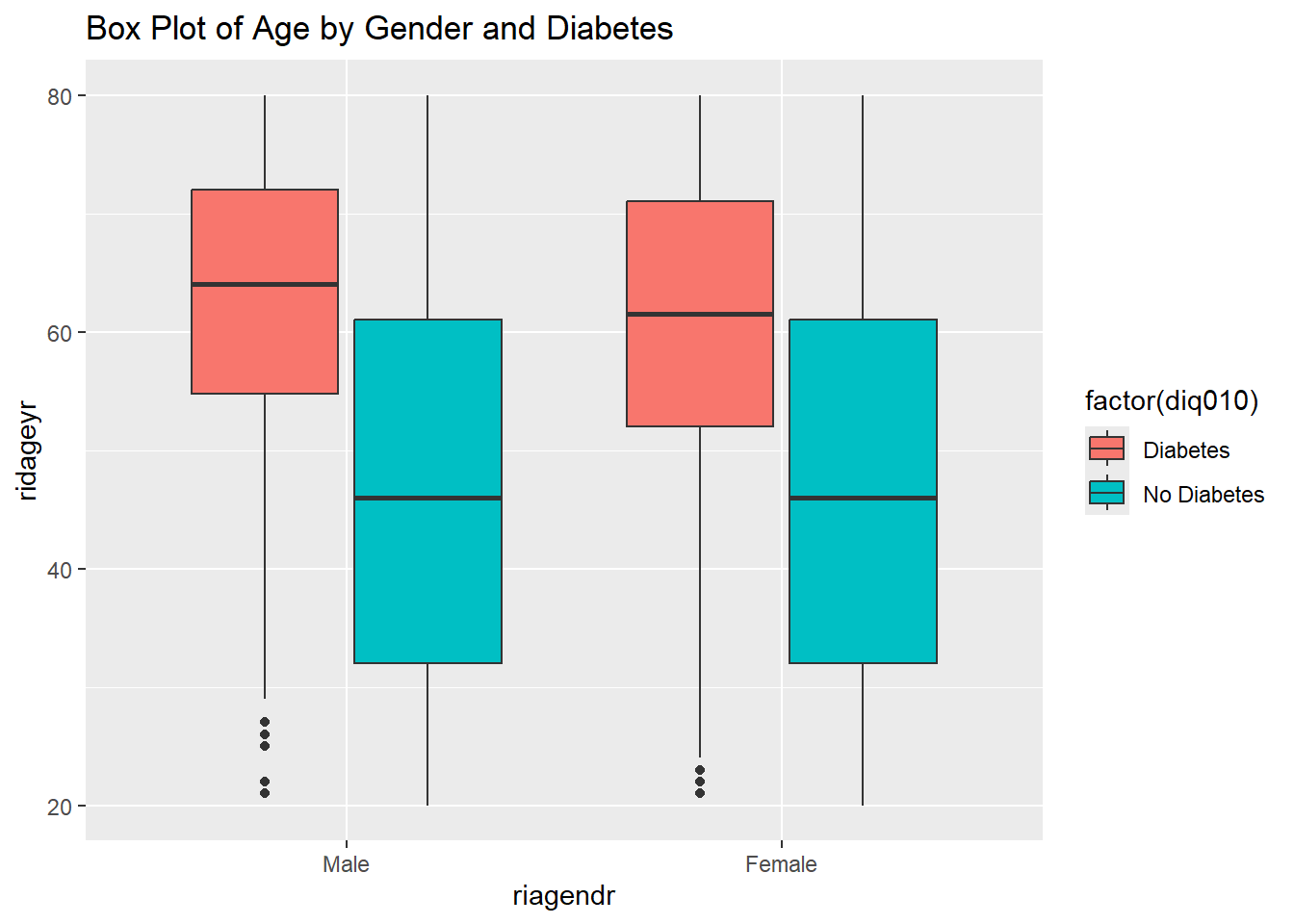
ggplot(diab_pop, aes(diq010,ridageyr)) +
  geom_boxplot(aes(fill=factor(diq010)))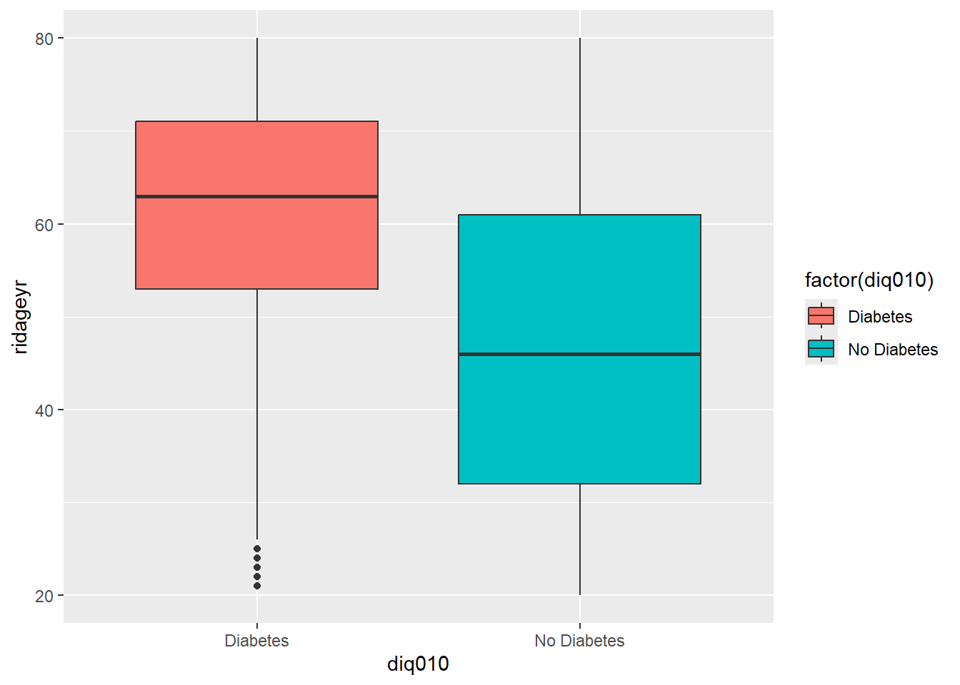
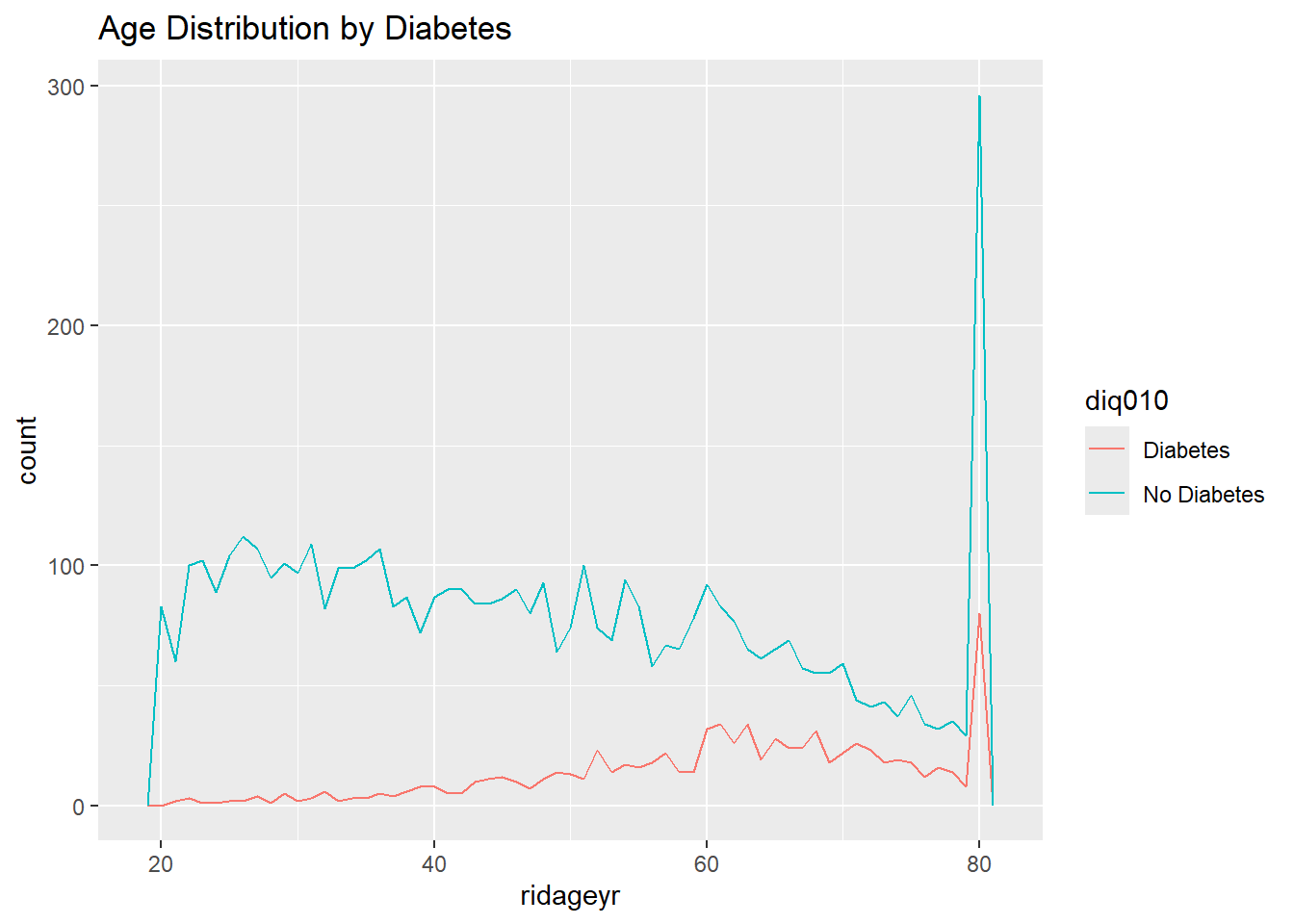
ggplot(diab_pop, aes(x=ridageyr)) + geom_histogram() + facet_wrap(~diq010)`stat_bin()` using `bins = 30`. Pick better value `binwidth`.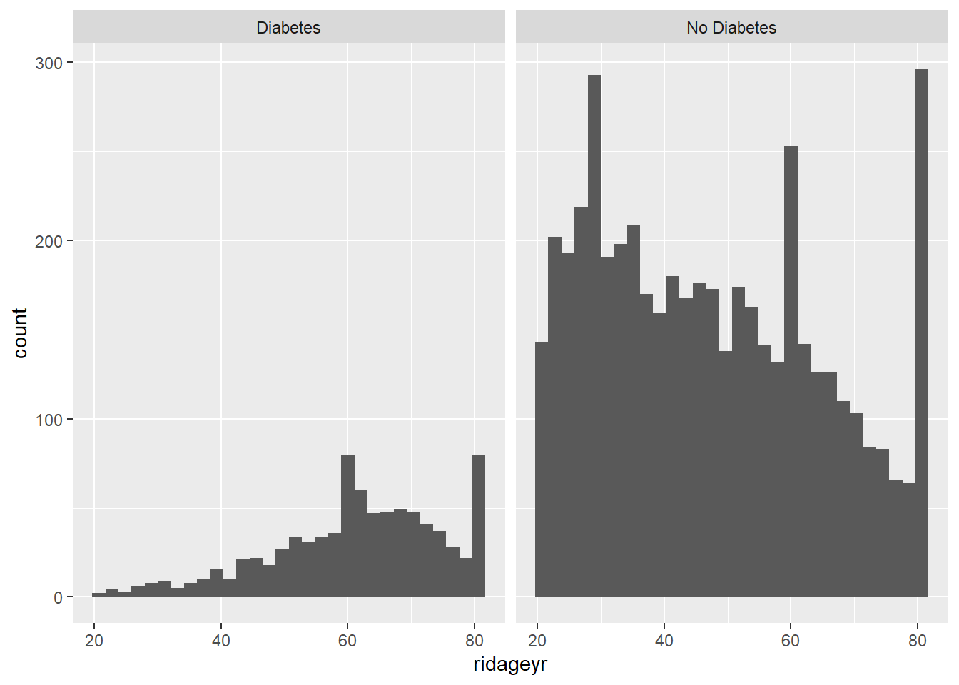
diab_pop.NoDm2 <- diab_pop %>% filter(diq010 == 'No Diabetes')
diab_pop.Dm2 <- diab_pop %>% filter(diq010 == 'Diabetes')

hist(diab_pop.NoDm2$ridageyr, col=rgb(1,0,0,0.5), main="Overlapping Histograms Diabetics by Age", xlab="Age")
hist(diab_pop.Dm2$ridageyr, col=rgb(0,0,1,0.5), add=T)
legend("topright", c("No Diabetes", "Diabetes"), fill=c(rgb(1,0,0,0.5), rgb(0,0,1,0.5)))
box()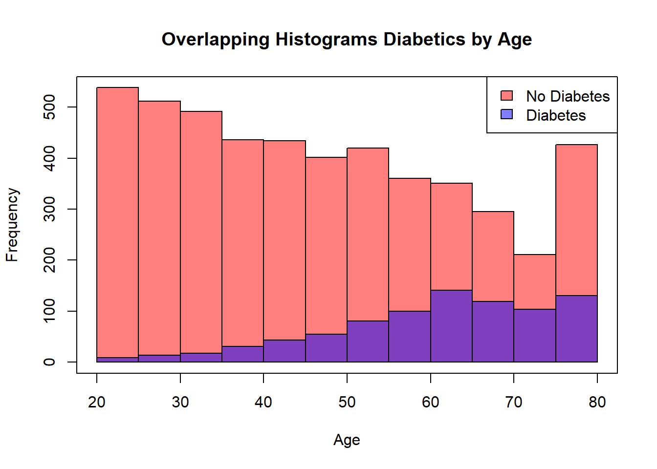
4.17.1 addition resources
- programming with
purrrvignette: https://purrr.tidyverse.org/ -
purrrcheatsheet: https://github.com/rstudio/cheatsheets/blob/master/purrr.pdf - kableExtra : https://cran.r-project.org/web/packages/kableExtra/vignettes/awesome_table_in_html.html
4.18 tableone
install_if_not('tableone')[1] "the package 'tableone' is already installed" Stratified by diq010
Diabetes No Diabetes p test
n 844 4875
ridageyr (mean (SD)) 61.34 (13.35) 47.49 (17.64) <0.001
bmxbmi (mean (SD)) 32.60 (7.73) 29.02 (6.82) <0.001
lbxglu (mean (SD)) 165.99 (73.48) 103.94 (20.72) <0.001
riagendr = Female (%) 388 (46.0) 2584 (53.0) <0.001
age_ntile (%) <0.001
1 58 ( 6.9) 1849 (37.9)
2 260 (30.8) 1646 (33.8)
3 526 (62.3) 1380 (28.3) 4.18.1 tableone - Additional Resources
- tableone vignette: https://cran.r-project.org/web/packages/tableone/vignettes/introduction.html
4.19 tableby with arsenal
install_if_not(c('arsenal','knitr','kableExtra'))[1] "the package 'arsenal' is already installed"
[2] "the package 'knitr' is already installed"
[3] "the package 'kableExtra' is already installed"
Attaching package: 'arsenal'The following object is masked from 'package:lubridate':
is.Datelibrary('knitr')
library('kableExtra')
table_arsenal <- tableby(diq010 ~ riagendr + dmdmartl, data = diab_pop)
table_arsenaltableby Object
Function Call:
tableby(formula = diq010 ~ riagendr + dmdmartl, data = diab_pop)
Variable(s):
diq010 ~ riagendr, dmdmartlsummary(table_arsenal, title="Diabetes by Sex and Marital Status")
Table: Diabetes by Sex and Marital Status
| | Diabetes (N=844) | No Diabetes (N=4875) | Total (N=5719) | p value|
|:-------------------------------------|:----------------:|:--------------------:|:--------------:|-------:|
|**riagendr** | | | | < 0.001|
| Male | 456 (54.0%) | 2291 (47.0%) | 2747 (48.0%) | |
| Female | 388 (46.0%) | 2584 (53.0%) | 2972 (52.0%) | |
|**dmdmartl** | | | | < 0.001|
| N-Miss | 0 | 3 | 3 | |
| Married | 471 (55.8%) | 2415 (49.6%) | 2886 (50.5%) | |
| Widowed | 100 (11.8%) | 321 (6.6%) | 421 (7.4%) | |
| Divorced | 106 (12.6%) | 508 (10.4%) | 614 (10.7%) | |
| Separated | 29 (3.4%) | 163 (3.3%) | 192 (3.4%) | |
| Never married | 83 (9.8%) | 965 (19.8%) | 1048 (18.3%) | |
| Living with partner | 55 (6.5%) | 500 (10.3%) | 555 (9.7%) | |summary.table_arsenal <- summary(table_arsenal, title="Diabetes by Sex and Marital Status",results="asis") %>%
kable() %>%
kable_styling("striped")
summary.table_arsenal | Diabetes (N=844) | No Diabetes (N=4875) | Total (N=5719) | p value | |
|---|---|---|---|---|
| **riagendr** | < 0.001 | |||
| Male | 456 (54.0%) | 2291 (47.0%) | 2747 (48.0%) | |
| Female | 388 (46.0%) | 2584 (53.0%) | 2972 (52.0%) | |
| **dmdmartl** | < 0.001 | |||
| N-Miss | 0 | 3 | 3 | |
| Married | 471 (55.8%) | 2415 (49.6%) | 2886 (50.5%) | |
| Widowed | 100 (11.8%) | 321 (6.6%) | 421 (7.4%) | |
| Divorced | 106 (12.6%) | 508 (10.4%) | 614 (10.7%) | |
| Separated | 29 (3.4%) | 163 (3.3%) | 192 (3.4%) | |
| Never married | 83 (9.8%) | 965 (19.8%) | 1048 (18.3%) | |
| Living with partner | 55 (6.5%) | 500 (10.3%) | 555 (9.7%) |
4.19.1 tableby - Additional Resources
- tableby vignette: https://cran.r-project.org/web/packages/arsenal/vignettes/tableby.html
4.20 anova
4.21 manova
            Df  Pillai approx F num Df den Df    Pr(>F)
diq010       1 0.10247   308.43      2   5403 < 2.2e-16 ***
Residuals 5404
---
Signif. codes: 0 '***' 0.001 '**' 0.01 '*' 0.05 '.' 0.1 ' ' 1summary.aov(res.mov) Response ridageyr :
Df Sum Sq Mean Sq F value Pr(>F)
diq010 1 122870 122870 425.86 < 2.2e-16 ***
Residuals 5404 1559176 289
---
Signif. codes: 0 '***' 0.001 '**' 0.01 '*' 0.05 '.' 0.1 ' ' 1
Response bmxbmi :
Df Sum Sq Mean Sq F value Pr(>F)
diq010 1 8619 8619.1 177.74 < 2.2e-16 ***
Residuals 5404 262052 48.5
---
Signif. codes: 0 '***' 0.001 '**' 0.01 '*' 0.05 '.' 0.1 ' ' 1
313 observations deleted due to missingness4.22 psych package
install_if_not("psych")[1] "the package 'psych' is already installed"psych::describe(diab_pop) vars n mean sd median trimmed mad min max
seqn 1 5719 88671.71 2877.82 88651.0 88662.57 3703.53 83732.0 93702.0
riagendr* 2 5719 1.52 0.50 2.0 1.52 0.00 1.0 2.0
ridageyr 3 5719 49.54 17.76 49.0 49.19 22.24 20.0 80.0
ridreth1* 4 5719 3.04 1.29 3.0 3.05 1.48 1.0 5.0
dmdeduc2* 5 5714 3.43 1.30 4.0 3.54 1.48 1.0 5.0
dmdmartl* 6 5716 2.61 1.89 1.0 2.39 0.00 1.0 6.0
indhhin2* 7 4421 8.47 4.32 8.0 8.59 5.93 1.0 14.0
bmxbmi 8 5406 29.54 7.08 28.5 28.86 6.38 14.5 67.3
diq010* 9 5719 1.85 0.35 2.0 1.94 0.00 1.0 2.0
lbxglu 10 2452 113.61 41.33 103.0 105.08 13.34 21.0 479.0
range skew kurtosis se
seqn 9970.0 0.02 -1.20 38.05
riagendr* 1.0 -0.08 -1.99 0.01
ridageyr 60.0 0.11 -1.14 0.23
ridreth1* 4.0 -0.12 -0.96 0.02
dmdeduc2* 4.0 -0.49 -0.84 0.02
dmdmartl* 5.0 0.63 -1.26 0.03
indhhin2* 13.0 -0.03 -1.46 0.06
bmxbmi 52.8 1.12 2.01 0.10
diq010* 1.0 -1.99 1.95 0.00
lbxglu 458.0 3.98 20.33 0.83
Attaching package: 'psych'The following objects are masked from 'package:ggplot2':
%+%, alphadescribeBy(diab_pop, diab_pop$diq010, skew=FALSE, ranges=TRUE)
 Descriptive statistics by group
group: Diabetes
         vars   n     mean      sd  median   min     max  range    se
seqn        1 844 88574.35 2845.20 88610.0 83732 93689.0 9957.0 97.94
riagendr    2 844     1.46    0.50     1.0     1     2.0    1.0  0.02
ridageyr    3 844    61.34   13.35    63.0    21    80.0   59.0  0.46
ridreth1    4 844     2.87    1.35     3.0     1     5.0    4.0  0.05
dmdeduc2    5 843     3.09    1.37     3.0     1     5.0    4.0  0.05
dmdmartl    6 844     2.19    1.65     1.0     1     6.0    5.0  0.06
indhhin2    7 650     7.24    4.23     6.0     1    14.0   13.0  0.17
bmxbmi      8 789    32.60    7.73    31.4    16    67.3   51.3  0.28
diq010      9 844     1.00    0.00     1.0     1     1.0    0.0  0.00
lbxglu     10 382   165.99   73.48   147.0    21   479.0  458.0  3.76
------------------------------------------------------------
group: No Diabetes
         vars    n     mean      sd median     min     max  range    se
seqn        1 4875 88688.57 2883.38  88654 83733.0 93702.0 9969.0 41.30
riagendr    2 4875     1.53    0.50      2     1.0     2.0    1.0  0.01
ridageyr    3 4875    47.49   17.64     46    20.0    80.0   60.0  0.25
ridreth1    4 4875     3.07    1.28      3     1.0     5.0    4.0  0.02
dmdeduc2    5 4871     3.49    1.28      4     1.0     5.0    4.0  0.02
dmdmartl    6 4872     2.68    1.92      2     1.0     6.0    5.0  0.03
indhhin2    7 3771     8.68    4.30      8     1.0    14.0   13.0  0.07
bmxbmi      8 4617    29.02    6.82     28    14.5    64.6   50.1  0.10
diq010      9 4875     2.00    0.00      2     2.0     2.0    0.0  0.00
lbxglu 10 2070 103.94 20.72 101 64.0 397.0 333.0 0.46detach(package:psych)4.22.1 psych - Additional Resources
- Into to psych : https://rdrr.io/cran/psych/f/inst/doc/intro.pdf
4.23 GGally::ggpairs
install_if_not('GGally')[1] "the package 'GGally' is already installed"`stat_bin()` using `bins = 30`. Pick better value `binwidth`.
`stat_bin()` using `bins = 30`. Pick better value `binwidth`.
`stat_bin()` using `bins = 30`. Pick better value `binwidth`.
`stat_bin()` using `bins = 30`. Pick better value `binwidth`.
`stat_bin()` using `bins = 30`. Pick better value `binwidth`.
`stat_bin()` using `bins = 30`. Pick better value `binwidth`.
`stat_bin()` using `bins = 30`. Pick better value `binwidth`.
`stat_bin()` using `bins = 30`. Pick better value `binwidth`.
`stat_bin()` using `bins = 30`. Pick better value `binwidth`.
`stat_bin()` using `bins = 30`. Pick better value `binwidth`.
`stat_bin()` using `bins = 30`. Pick better value `binwidth`.
`stat_bin()` using `bins = 30`. Pick better value `binwidth`.
`stat_bin()` using `bins = 30`. Pick better value `binwidth`.
`stat_bin()` using `bins = 30`. Pick better value `binwidth`.
`stat_bin()` using `bins = 30`. Pick better value `binwidth`.
`stat_bin()` using `bins = 30`. Pick better value `binwidth`.
`stat_bin()` using `bins = 30`. Pick better value `binwidth`.
`stat_bin()` using `bins = 30`. Pick better value `binwidth`.
`stat_bin()` using `bins = 30`. Pick better value `binwidth`.
`stat_bin()` using `bins = 30`. Pick better value `binwidth`.
`stat_bin()` using `bins = 30`. Pick better value `binwidth`.
`stat_bin()` using `bins = 30`. Pick better value `binwidth`.
`stat_bin()` using `bins = 30`. Pick better value `binwidth`.
`stat_bin()` using `bins = 30`. Pick better value `binwidth`.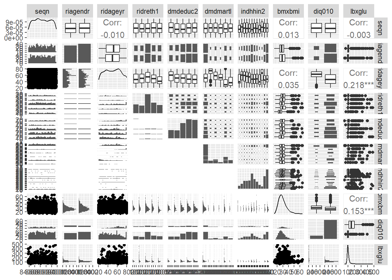
4.24 skimr
install_if_not('skimr')[1] "the package 'skimr' is already installed"| Name | diab_pop |
| Number of rows | 5719 |
| Number of columns | 10 |
| _______________________ | |
| Column type frequency: | |
| factor | 6 |
| numeric | 4 |
| ________________________ | |
| Group variables | None |
skim(diab_pop) | Name | diab_pop |
| Number of rows | 5719 |
| Number of columns | 10 |
| _______________________ | |
| Column type frequency: | |
| factor | 6 |
| numeric | 4 |
| ________________________ | |
| Group variables | None |
Variable type: factor
| skim_variable | n_missing | complete_rate | ordered | n_unique | top_counts |
|---|---|---|---|---|---|
| riagendr | 0 | 1.00 | FALSE | 2 | Fem: 2972, Mal: 2747 |
| ridreth1 | 0 | 1.00 | FALSE | 5 | Non: 1863, Non: 1198, Mex: 995, Oth: 895 |
| dmdeduc2 | 5 | 1.00 | FALSE | 5 | Som: 1692, Col: 1422, Hig: 1236, Les: 688 |
| dmdmartl | 3 | 1.00 | FALSE | 6 | Mar: 2886, Nev: 1048, Div: 614, Liv: 555 |
| indhhin2 | 1298 | 0.77 | FALSE | 12 | $10: 910, $25: 596, $75: 524, $45: 451 |
| diq010 | 0 | 1.00 | FALSE | 2 | No : 4875, Dia: 844 |
Variable type: numeric
| skim_variable | n_missing | complete_rate | mean | sd | p0 | p25 | p50 | p75 | p100 | hist |
|---|---|---|---|---|---|---|---|---|---|---|
| seqn | 0 | 1.00 | 88671.71 | 2877.82 | 83732.0 | 86170.5 | 88651.0 | 91165.5 | 93702.0 | ▇▇▇▇▇ |
| ridageyr | 0 | 1.00 | 49.54 | 17.76 | 20.0 | 34.0 | 49.0 | 64.0 | 80.0 | ▇▇▇▇▆ |
| bmxbmi | 313 | 0.95 | 29.54 | 7.08 | 14.5 | 24.5 | 28.5 | 33.2 | 67.3 | ▅▇▂▁▁ |
| lbxglu | 3267 | 0.43 | 113.61 | 41.33 | 21.0 | 95.0 | 103.0 | 114.0 | 479.0 | ▇▂▁▁▁ |
| Name | Piped data |
| Number of rows | 5719 |
| Number of columns | 10 |
| _______________________ | |
| Column type frequency: | |
| factor | 5 |
| numeric | 4 |
| ________________________ | |
| Group variables | diq010 |
Variable type: factor
| skim_variable | diq010 | n_missing | complete_rate | ordered | n_unique | top_counts |
|---|---|---|---|---|---|---|
| riagendr | Diabetes | 0 | 1.00 | FALSE | 2 | Mal: 456, Fem: 388 |
| riagendr | No Diabetes | 0 | 1.00 | FALSE | 2 | Fem: 2584, Mal: 2291 |
| ridreth1 | Diabetes | 0 | 1.00 | FALSE | 5 | Non: 217, Non: 203, Mex: 200, Oth: 119 |
| ridreth1 | No Diabetes | 0 | 1.00 | FALSE | 5 | Non: 1646, Non: 995, Mex: 795, Oth: 790 |
| dmdeduc2 | Diabetes | 1 | 1.00 | FALSE | 5 | Som: 229, Hig: 185, Les: 161, Col: 145 |
| dmdeduc2 | No Diabetes | 4 | 1.00 | FALSE | 5 | Som: 1463, Col: 1277, Hig: 1051, Gra: 553 |
| dmdmartl | Diabetes | 0 | 1.00 | FALSE | 6 | Mar: 471, Div: 106, Wid: 100, Nev: 83 |
| dmdmartl | No Diabetes | 3 | 1.00 | FALSE | 6 | Mar: 2415, Nev: 965, Div: 508, Liv: 500 |
| indhhin2 | Diabetes | 194 | 0.77 | FALSE | 12 | $10: 89, $25: 86, $10: 81, $20: 68 |
| indhhin2 | No Diabetes | 1104 | 0.77 | FALSE | 12 | $10: 821, $25: 510, $75: 472, $45: 386 |
Variable type: numeric
| skim_variable | diq010 | n_missing | complete_rate | mean | sd | p0 | p25 | p50 | p75 | p100 | hist |
|---|---|---|---|---|---|---|---|---|---|---|---|
| seqn | Diabetes | 0 | 1.00 | 88574.35 | 2845.20 | 83732.0 | 86068.75 | 88610.0 | 90994.5 | 93689.0 | ▇▇▇▇▇ |
| seqn | No Diabetes | 0 | 1.00 | 88688.57 | 2883.38 | 83733.0 | 86189.50 | 88654.0 | 91193.0 | 93702.0 | ▇▇▇▇▇ |
| ridageyr | Diabetes | 0 | 1.00 | 61.34 | 13.35 | 21.0 | 53.00 | 63.0 | 71.0 | 80.0 | ▁▂▅▇▇ |
| ridageyr | No Diabetes | 0 | 1.00 | 47.49 | 17.64 | 20.0 | 32.00 | 46.0 | 61.0 | 80.0 | ▇▇▆▆▅ |
| bmxbmi | Diabetes | 55 | 0.93 | 32.60 | 7.73 | 16.0 | 27.40 | 31.4 | 36.3 | 67.3 | ▂▇▂▁▁ |
| bmxbmi | No Diabetes | 258 | 0.95 | 29.02 | 6.82 | 14.5 | 24.10 | 28.0 | 32.5 | 64.6 | ▃▇▂▁▁ |
| lbxglu | Diabetes | 462 | 0.45 | 165.99 | 73.48 | 21.0 | 117.00 | 147.0 | 192.0 | 479.0 | ▃▇▂▁▁ |
| lbxglu | No Diabetes | 2805 | 0.42 | 103.94 | 20.72 | 64.0 | 94.00 | 101.0 | 109.0 | 397.0 | ▇▁▁▁▁ |
4.25 Sankey Network
install_if_not('networkD3')[1] "the package 'networkD3' is already installed"`summarise()` has regrouped the output.
ℹ Summaries were computed grouped by riagendr and ridreth1.
ℹ Output is grouped by riagendr.
ℹ Use `summarise(.groups = "drop_last")` to silence this message.
ℹ Use `summarise(.by = c(riagendr, ridreth1))` for per-operation grouping
(`?dplyr::dplyr_by`) instead.by_sex_by_dm2 <- diab_pop %>%
group_by(riagendr, diq010) %>%
summarise(cnt = n_distinct(seqn))`summarise()` has regrouped the output.
ℹ Summaries were computed grouped by riagendr and diq010.
ℹ Output is grouped by riagendr.
ℹ Use `summarise(.groups = "drop_last")` to silence this message.
ℹ Use `summarise(.by = c(riagendr, diq010))` for per-operation grouping
(`?dplyr::dplyr_by`) instead.join1 <- by_sex %>%
left_join(by_sex_by_eth,
by= c('riagendr'='riagendr'),
suffix = c("_sex","_eth")) %>%
mutate(diff_sex_eth = cnt_sex - cnt_eth) %>%
mutate(source = riagendr,
target = ridreth1) %>%
mutate(diff = diff_sex_eth) %>%
select(source, target, diff)
join2 <- by_sex %>%
left_join(by_sex_by_dm2,
by= c('riagendr'='riagendr'),
suffix = c("_sex","_dm2")) %>%
mutate(diff_sex_dm2 = cnt_sex - cnt_dm2 )%>%
mutate(source = riagendr,
target = diq010) %>%
mutate(diff = diff_sex_dm2)%>%
select(source, target, diff)
by_dm2 <-diab_pop %>%
group_by(diq010)%>%
summarise(cnt = n_distinct(seqn))
by_dm2_by_eth <-diab_pop %>%
group_by(diq010, ridreth1)%>%
summarise(cnt = n_distinct(seqn))`summarise()` has regrouped the output.
ℹ Summaries were computed grouped by diq010 and ridreth1.
ℹ Output is grouped by diq010.
ℹ Use `summarise(.groups = "drop_last")` to silence this message.
ℹ Use `summarise(.by = c(diq010, ridreth1))` for per-operation grouping
(`?dplyr::dplyr_by`) instead.join3 <- by_dm2 %>%
left_join(by_dm2_by_eth,
by= c('diq010'='diq010'),
suffix = c("_dm2","_eth")) %>%
mutate(diff_dm2_eth = cnt_dm2 - cnt_eth) %>%
mutate(source = ridreth1,
target = diq010) %>%
mutate(diff = diff_dm2_eth) %>%
select(source, target, diff)
JOIN <- bind_rows(join1, join2, join3)
nodes <- data.frame(
name=c( as.character(JOIN$source),
as.character(JOIN$target))
%>% unique()
)
JOIN$IDsource <- match(JOIN$source, nodes$name)-1
JOIN$IDtarget <- match(JOIN$target, nodes$name)-1
p <- sankeyNetwork(Links = JOIN,
Nodes = nodes,
Source = "IDsource",
Target = "IDtarget",
Value = "diff",
NodeID = "name",
sinksRight=FALSE)Links is a tbl_df. Converting to a plain data frame.p
4.25.1 Additional Sankey Network resources:
- Wikipedia Sankey Diagram - https://en.wikipedia.org/wiki/Sankey_diagram
- Other resources - https://www.r-graph-gallery.com/sankey-diagram.html
- Automated Sankey on a Feature Set - https://rpubs.com/jkylearmstrong/Automated_Sankey_Network_Diagram_Example