25  Random Forest Imputation and Multi-class Classifier

\(~\)

\(~\)

25.1 NHANES data

library('tidyverse')

── Attaching core tidyverse packages ──────────────────────── tidyverse 2.0.0 ──
✔ dplyr     1.2.1     ✔ readr     2.2.0
✔ forcats   1.0.1     ✔ stringr   1.6.0
✔ ggplot2   4.0.3     ✔ tibble    3.3.1
✔ lubridate 1.9.5     ✔ tidyr     1.3.2
✔ purrr     1.2.2     
── Conflicts ────────────────────────────────────────── tidyverse_conflicts() ──
✖ dplyr::filter() masks stats::filter()
✖ dplyr::lag()    masks stats::lag()
ℹ Use the conflicted package (<http://conflicted.r-lib.org/>) to force all conflicts to become errors

library(NHANES)

NHANES_DATA_12 <- NHANES %>%
  filter(!is.na(Depressed))

25.1.1 Note that Depressed is has 3 potiential classes

NHANES_DATA_12 %>% 
  select(Depressed) %>%
  distinct()

# A tibble: 3 × 1
  Depressed
  <fct>    
1 Several  
2 None     
3 Most     

\(~\)

\(~\)

---

\(~\)

\(~\)

25.2 Some data prep

SumNa <- function(col){sum(is.na(col))}

data.sum <- NHANES_DATA_12 %>% 
  summarise_all(SumNa) %>%
  tidyr::gather(key='feature', value='SumNa') %>%
  arrange(-SumNa) %>%
  mutate(PctNa = SumNa/nrow(NHANES_DATA_12))

data.sum2 <- data.sum %>% 
  filter(! (feature %in% c('ID','Depressed'))) %>%
  filter(PctNa < .85)

data.sum2$feature

 [1] "UrineFlow2"      "UrineVol2"       "AgeRegMarij"     "PregnantNow"    
 [5] "Age1stBaby"      "nBabies"         "nPregnancies"    "SmokeAge"       
 [9] "AgeFirstMarij"   "SmokeNow"        "Testosterone"    "AgeMonths"      
[13] "TVHrsDay"        "Race3"           "CompHrsDay"      "PhysActiveDays" 
[17] "SexOrientation"  "AlcoholDay"      "SexNumPartYear"  "Marijuana"      
[21] "RegularMarij"    "SexAge"          "SexNumPartnLife" "HardDrugs"      
[25] "SexEver"         "SameSex"         "AlcoholYear"     "HHIncome"       
[29] "HHIncomeMid"     "Poverty"         "UrineFlow1"      "BPSys1"         
[33] "BPDia1"          "AgeDecade"       "DirectChol"      "TotChol"        
[37] "BPSys2"          "BPDia2"          "Education"       "BPSys3"         
[41] "BPDia3"          "MaritalStatus"   "Smoke100"        "Smoke100n"      
[45] "Alcohol12PlusYr" "BPSysAve"        "BPDiaAve"        "Pulse"          
[49] "BMI_WHO"         "BMI"             "Weight"          "HomeRooms"      
[53] "Height"          "HomeOwn"         "UrineVol1"       "SleepHrsNight"  
[57] "LittleInterest"  "DaysPhysHlthBad" "DaysMentHlthBad" "Diabetes"       
[61] "Work"            "SurveyYr"        "Gender"          "Age"            
[65] "Race1"           "HealthGen"       "SleepTrouble"    "PhysActive"     

data_F <- NHANES_DATA_12 %>% 
  select(ID, Depressed, data.sum2$feature) %>%
  filter(!is.na(Depressed))

25.2.1 note that data_F still has missing values

Amelia::missmap(as.data.frame(data_F))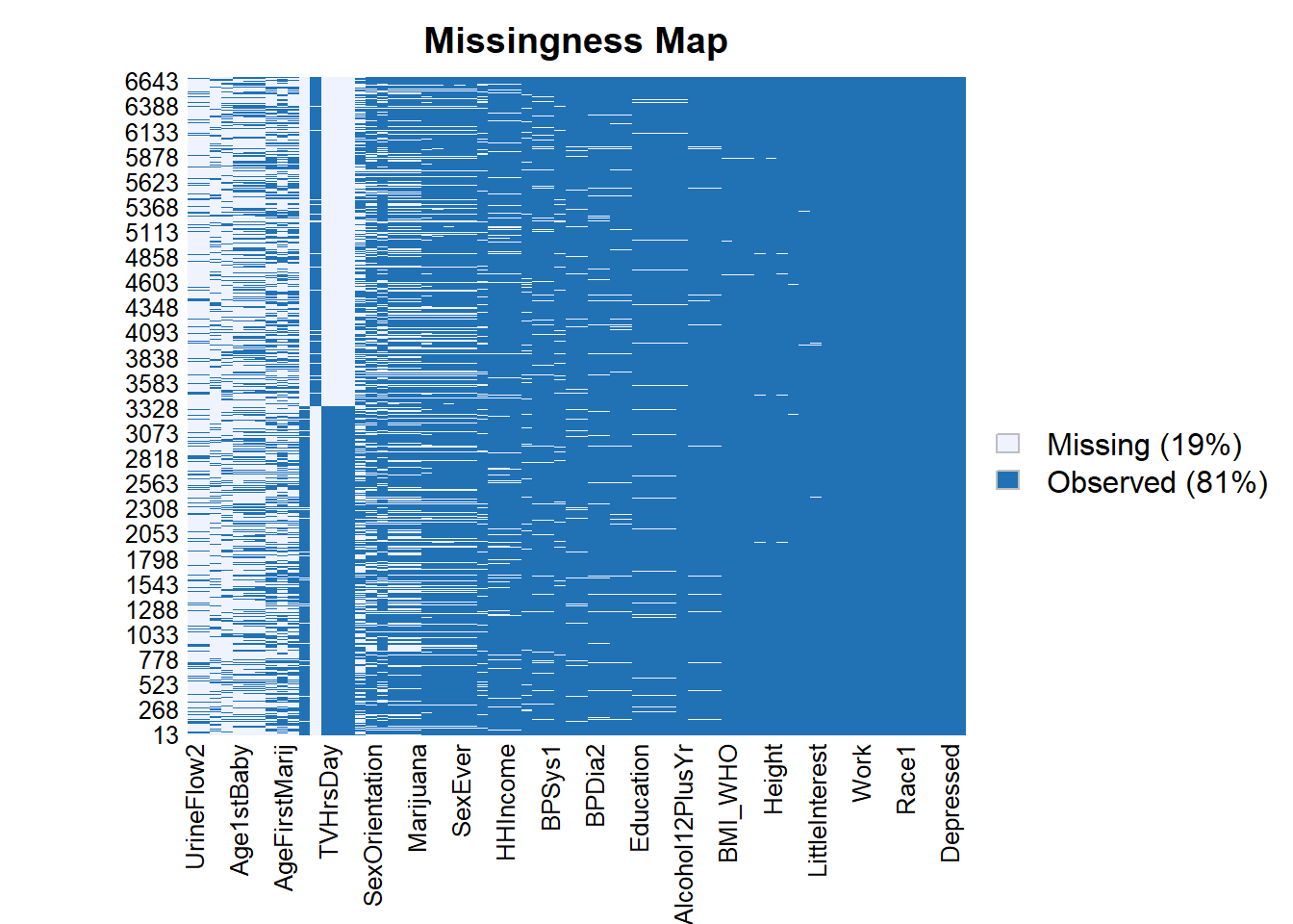

\(~\)

\(~\)

---

\(~\)

\(~\)

25.3 Random Forest Impute with rfImpute

library('randomForest')

randomForest 4.7-1.2

Type rfNews() to see new features/changes/bug fixes.

Attaching package: 'randomForest'

The following object is masked from 'package:dplyr':

    combine

The following object is masked from 'package:ggplot2':

    margin

data_F.imputed <- rfImpute(Depressed ~ . , 
                           data_F, 
                           iter=2, 
                           ntree=300)

ntree      OOB      1      2      3
  300:   8.24%  0.80% 36.27% 33.97%
ntree      OOB      1      2      3
  300:   8.56%  1.20% 36.57% 33.25%

25.3.0.1 Note we no longer have missing data

Amelia::missmap(as.data.frame(data_F.imputed))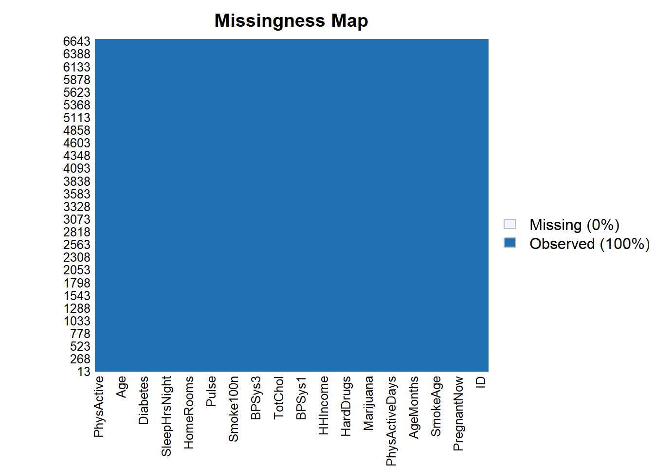

\(~\)

\(~\)

---

\(~\)

\(~\)

25.4 Split Data

library('caret')

Loading required package: lattice

Attaching package: 'caret'

The following object is masked from 'package:purrr':

    lift

set.seed(8576309)

trainIndex <- createDataPartition(data_F.imputed$Depressed, 
                                  p = .6, 
                                  list = FALSE, 
                                  times = 1)

TRAIN <- data_F.imputed[trainIndex, ]
TEST <- data_F.imputed[-trainIndex, ]

\(~\)

\(~\)

---

\(~\)

\(~\)

25.5 Train model

train_ctrl <- trainControl(method="cv", # type of resampling in this case Cross-Validated
                           number=3, # number of folds
                           search = "random", # we are performing a "random
                           )

toc <- Sys.time()
model_rf <- train(Depressed ~ .,
                       data = TRAIN,
                       method = "rf", # this will use the randomForest::randomForest function
                       metric = "Accuracy", # which metric should be optimized for 
                       trControl = train_ctrl,
                       # options to be passed to randomForest
                       ntree = 741,
                       keep.forest=TRUE,
                       importance=TRUE) 
tic <- Sys.time()

tic - toc

Time difference of 3.846963 mins

25.5.1 Model output

model_rf

Random Forest 

4005 samples
  69 predictor
   3 classes: 'None', 'Several', 'Most' 

No pre-processing
Resampling: Cross-Validated (3 fold) 
Summary of sample sizes: 2670, 2669, 2671 
Resampling results across tuning parameters:

  mtry  Accuracy   Kappa    
  11    0.8786518  0.5936139
  63    0.8896379  0.6603935
  75    0.8858937  0.6493560

Accuracy was used to select the optimal model using the largest value.
The final value used for the model was mtry = 63.

randomForest::varImpPlot(model_rf$finalModel)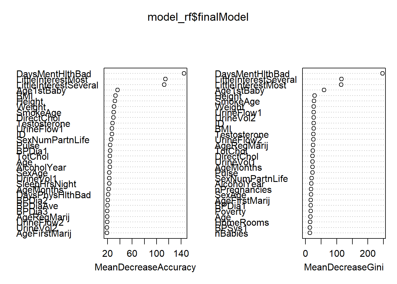

\(~\)

\(~\)

---

\(~\)

\(~\)

25.6 Score Test Data

probs <- predict(model_rf, TEST, 'prob')
class <- predict(model_rf, TEST, 'raw')


TEST.scored <- cbind(TEST, probs, class)

25.6.1 Use yardstick for Model Metrics

library('yardstick')

Attaching package: 'yardstick'

The following objects are masked from 'package:caret':

    precision, recall, sensitivity, specificity

The following object is masked from 'package:readr':

    spec

cm <- conf_mat(TEST.scored, truth = Depressed, class)

cm

          Truth
Prediction None Several Most
   None    2029     153   25
   Several   58     225   22
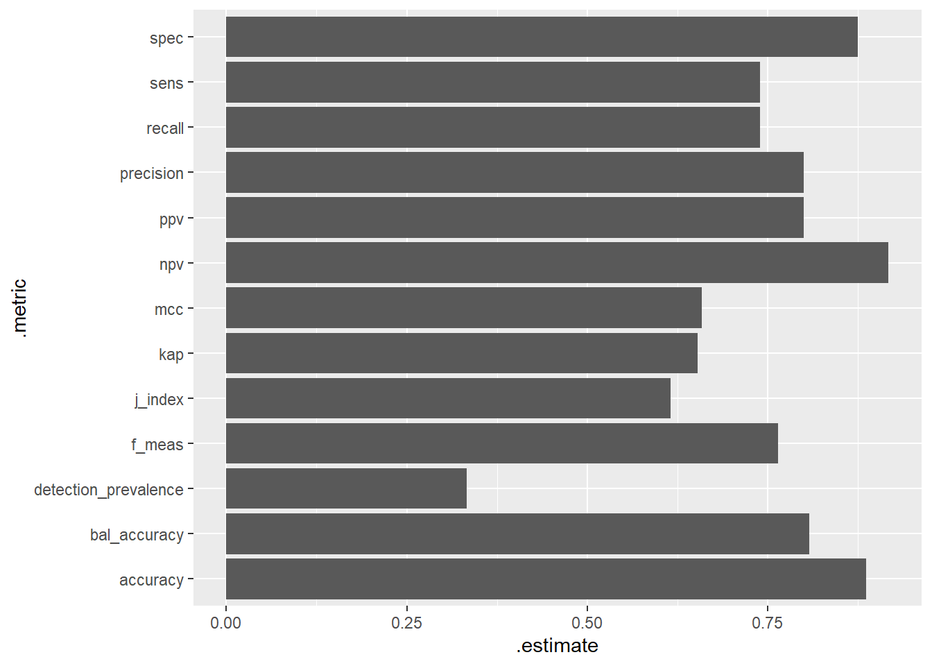
   Most      11      25  120

summary(cm)

# A tibble: 13 × 3
   .metric              .estimator .estimate
   <chr>                <chr>          <dbl>
 1 accuracy             multiclass     0.890
 2 kap                  multiclass     0.665
 3 sens                 macro          0.748
 4 spec                 macro          0.879
 5 ppv                  macro          0.809
 6 npv                  macro          0.919
 7 mcc                  multiclass     0.670
 8 j_index              macro          0.627
 9 bal_accuracy         macro          0.814
10 detection_prevalence macro          0.333
11 precision            macro          0.809
12 recall               macro          0.748
13 f_meas               macro          0.774

library('ggplot2')

ggplot(summary(cm), aes(x=.metric, y=.estimate)) + 
  geom_bar(stat="identity") + 
  coord_flip()