13  Linear Regression

13.1 Load data on the height and weight of school children


Attaching package: 'dplyr'
The following objects are masked from 'package:stats':

    filter, lag
The following objects are masked from 'package:base':
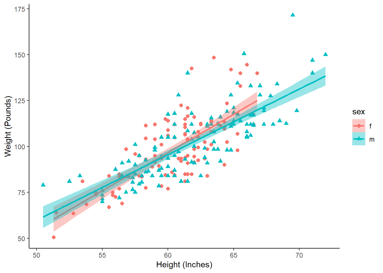
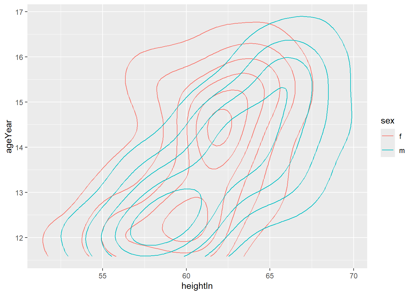
    intersect, setdiff, setequal, union
Loading required package: viridisLite
df <- gcookbook::heightweight

# Look at data

glimpse(df)
Rows: 236
Columns: 5
$ sex      <fct> f, f, f, f, f, f, f, f, f, f, f, f, f, f, f, f, f, f, f, f, f…
$ ageYear  <dbl> 11.92, 12.92, 12.75, 13.42, 15.92, 14.25, 15.42, 11.83, 13.33…
$ ageMonth <int> 143, 155, 153, 161, 191, 171, 185, 142, 160, 140, 139, 178, 1…
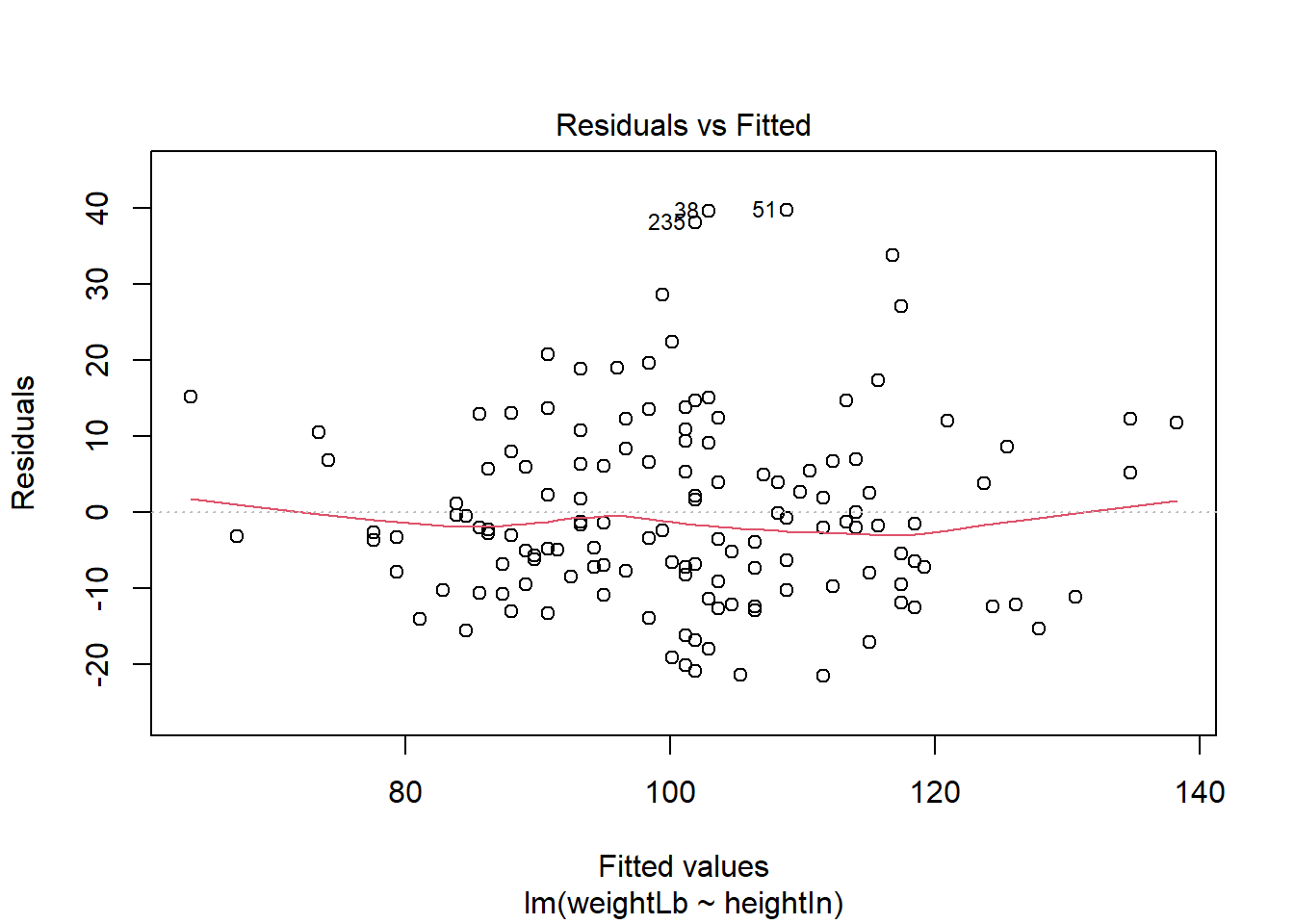
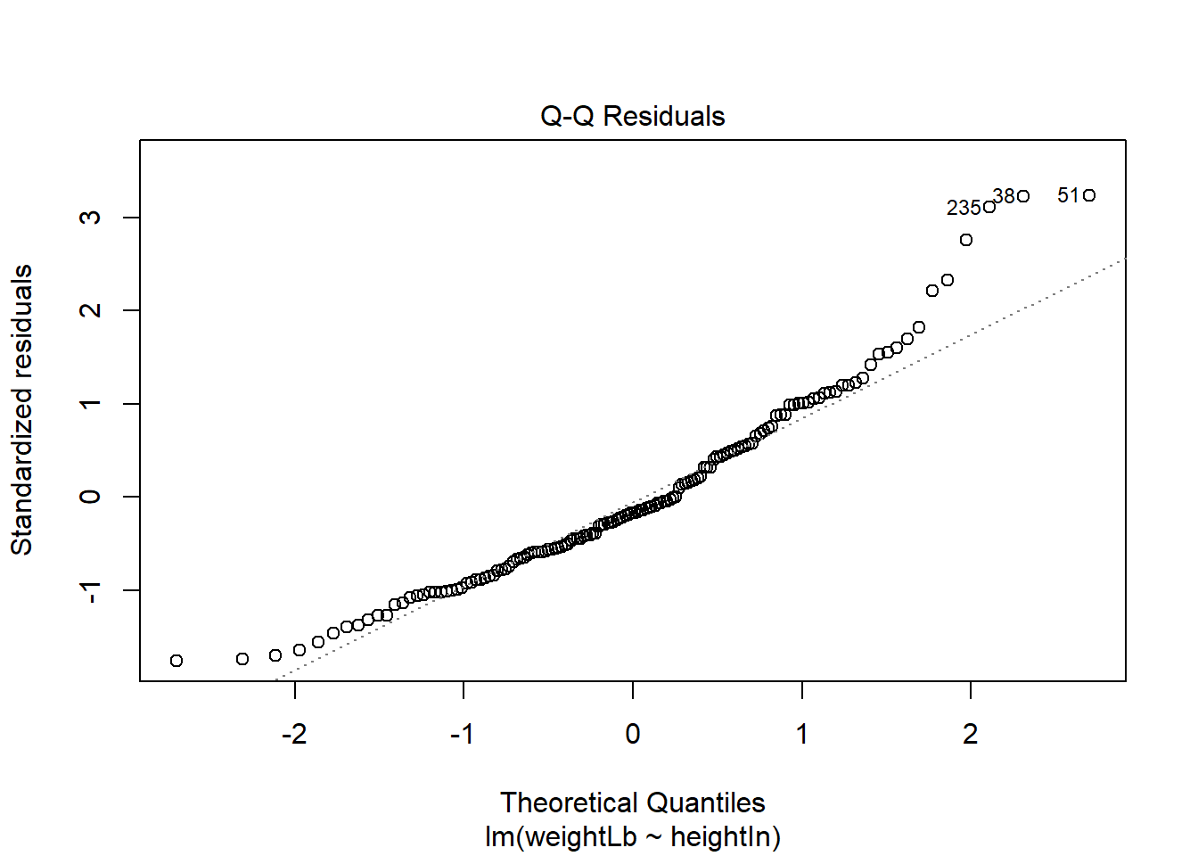
$ heightIn <dbl> 56.3, 62.3, 63.3, 59.0, 62.5, 62.5, 59.0, 56.5, 62.0, 53.8, 6…
$ weightLb <dbl> 85.0, 105.0, 108.0, 92.0, 112.5, 112.0, 104.0, 69.0, 94.5, 68…

13.2 Plots

13.2.1 Scatter plot showing the relationship between height and weight.

ggplot(aes(x = heightIn, y = weightLb, fill=sex, shape=sex, color=sex), data = df) + 
  geom_point(size = 2) + 
  stat_smooth(method="lm") + 
  theme_bw()+
  xlab("Height (Inches)")+
  #xlab("")+
  ylab("Weight (Pounds)")+
  #ylab("")+
  theme(panel.grid.minor = element_blank(),
        panel.grid.major = element_blank(),
        panel.border = element_blank(),
        axis.line.x = element_line(color="black"),
        axis.line.y = element_line(color="black"))
`geom_smooth()` using formula = 'y ~ x'

13.2.2 Contour plots

ggplot(df, aes(x=heightIn, y=ageYear, z=weightLb, color = sex)) + geom_density_2d()
Warning: The following aesthetics were dropped during statistical transformation: z.
ℹ This can happen when ggplot fails to infer the correct grouping structure in
  the data.
ℹ Did you forget to specify a `group` aesthetic or to convert a numerical
  variable into a factor?

13.3 Split Data into TRAIN and TEST

Loading required package: lattice
set.seed(85765309)

trainIndex <- createDataPartition(df$weightLb, p = .6, list=FALSE)
train <- df[trainIndex,]
test <- df[-trainIndex,]

13.4 Model 1 - simple linear regresssion

13.4.1 train the model

model1 <- lm(weightLb ~ heightIn, data=train)

13.4.2 model summary and plots

model1

Call:
lm(formula = weightLb ~ heightIn, data = train)

Coefficients:
(Intercept)     heightIn  
   -111.209        3.464  
summary(model1)

Call:
lm(formula = weightLb ~ heightIn, data = train)

Residuals:
    Min      1Q  Median      3Q     Max 
-21.546  -8.046  -2.055   6.788  39.725 

Coefficients:
             Estimate Std. Error t value Pr(>|t|)    
(Intercept) -111.2089    15.8801  -7.003 9.21e-11 ***
heightIn       3.4643     0.2583  13.414  < 2e-16 ***
---
Signif. codes:  0 '***' 0.001 '**' 0.01 '*' 0.05 '.' 0.1 ' ' 1

Residual standard error: 12.32 on 142 degrees of freedom
Multiple R-squared:  0.5589,    Adjusted R-squared:  0.5558 
F-statistic: 179.9 on 1 and 142 DF,  p-value: < 2.2e-16
plot(model1)

13.4.3 Score test - get predicted values

predicted <- predict(model1, test)
observed <- test$weightLb

13.4.4 Manually calculate mean squared error and root mean squared error

mse = mean( (predicted - observed)^2, na.rm = TRUE)
mse
[1] 132.1941
rmse = sqrt(mse)
rmse
[1] 11.49757

13.4.5 Use yardstick package and rmse function

test.scored <- cbind(test,predicted)

library('yardstick')

Attaching package: 'yardstick'
The following objects are masked from 'package:caret':

    precision, recall, sensitivity, specificity
RMSE <- rmse(test.scored, weightLb, predicted,  na_rm = TRUE)

RMSE
# A tibble: 1 × 3
  .metric .estimator .estimate
  <chr>   <chr>          <dbl>
1 rmse    standard        11.5
MSE <- RMSE$.estimate^2

MSE
[1] 132.1941

13.5 Model 2 - multiple linear regression model

13.5.1 Train multiple linear regression model

# Add in age
model2 <- lm(weightLb ~ heightIn + ageYear , data=train)

summary(model2)

Call:
lm(formula = weightLb ~ heightIn + ageYear, data = train)

Residuals:
    Min      1Q  Median      3Q     Max 
-22.991  -8.504  -2.382   6.618  38.106 

Coefficients:
             Estimate Std. Error t value Pr(>|t|)    
(Intercept) -112.6845    15.6695  -7.191 3.45e-11 ***
heightIn       3.0394     0.3166   9.600  < 2e-16 ***
ageYear        2.0280     0.8982   2.258   0.0255 *  
---
Signif. codes:  0 '***' 0.001 '**' 0.01 '*' 0.05 '.' 0.1 ' ' 1

Residual standard error: 12.15 on 141 degrees of freedom
Multiple R-squared:  0.5743,    Adjusted R-squared:  0.5683 
F-statistic: 95.11 on 2 and 141 DF,  p-value: < 2.2e-16
plot(model2)

13.5.2 Score Test

prediction2 <- predict(model2, test)

test.scored2 <- cbind(test,prediction2)

13.5.3 yardstick

# root mean squared error
rmse(test.scored2, weightLb, prediction2)
# A tibble: 1 × 3
  .metric .estimator .estimate
  <chr>   <chr>          <dbl>
1 rmse    standard        11.1
# mean absolute error
mae(test.scored2, weightLb, prediction2)
# A tibble: 1 × 3
  .metric .estimator .estimate
  <chr>   <chr>          <dbl>
1 mae     standard        8.82
# r^2 - Calculate the coefficient of determination using correlation.
rsq(test.scored2, weightLb, prediction2)
# A tibble: 1 × 3
  .metric .estimator .estimate
  <chr>   <chr>          <dbl>
1 rsq     standard       0.695
# r^2 - Calculate the coefficient of determination using the traditional definition of R squared using sum of squares.
rsq_trad(test.scored2, weightLb, prediction2)
# A tibble: 1 × 3
  .metric  .estimator .estimate
  <chr>    <chr>          <dbl>
1 rsq_trad standard       0.680

13.6 Model 3

model3 <- lm(weightLb ~ heightIn*sex + ageYear + I(ageYear^2) + sex + heightIn, data=train)

model3

Call:
lm(formula = weightLb ~ heightIn * sex + ageYear + I(ageYear^2) + 
    sex + heightIn, data = train)

Coefficients:
  (Intercept)       heightIn           sexm        ageYear   I(ageYear^2)  
      11.6227         3.2677        14.1932       -17.9445         0.7146  
heightIn:sexm  
      -0.2362  
summary(model3)

Call:
lm(formula = weightLb ~ heightIn * sex + ageYear + I(ageYear^2) + 
    sex + heightIn, data = train)

Residuals:
    Min      1Q  Median      3Q     Max 
-21.799  -8.270  -2.619   6.608  39.509 

Coefficients:
              Estimate Std. Error t value Pr(>|t|)    
(Intercept)    11.6227    96.9471   0.120    0.905    
heightIn        3.2677     0.5065   6.451 1.74e-09 ***
sexm           14.1932    34.6233   0.410    0.682    
ageYear       -17.9445    13.8948  -1.291    0.199    
I(ageYear^2)    0.7146     0.4964   1.440    0.152    
heightIn:sexm  -0.2362     0.5668  -0.417    0.677    
---
Signif. codes:  0 '***' 0.001 '**' 0.01 '*' 0.05 '.' 0.1 ' ' 1

Residual standard error: 12.18 on 138 degrees of freedom
Multiple R-squared:  0.5811,    Adjusted R-squared:  0.5659 
F-statistic: 38.29 on 5 and 138 DF,  p-value: < 2.2e-16
plot(model3)