install_if_not <- function( list.of.packages ) {
  new.packages <- list.of.packages[!(list.of.packages %in% installed.packages()[,"Package"])]
  if(length(new.packages)) { install.packages(new.packages) } else { print(paste0("the package '", list.of.packages , "' is already installed")) }
}26 Nested Cross-Validation Example
\(~\)
\(~\)
Install if not Function
\(~\)
\(~\)
\(~\)
26.1 Getting Started!
\(~\)
The rsample::initial_split function works similarly to the caret::createDataPartition function.
The rsample::training and rsample::testing functions will return back the training or testing data.
diab_pop <- readRDS(here::here('DATA','diab_pop.RDS'))

library('tidyverse')
── Attaching core tidyverse packages ──────────────────────── tidyverse 2.0.0 ──
✔ dplyr 1.2.1 ✔ readr 2.2.0
✔ forcats 1.0.1 ✔ stringr 1.6.0
✔ ggplot2 4.0.3 ✔ tibble 3.3.1
✔ lubridate 1.9.5 ✔ tidyr 1.3.2
✔ purrr 1.2.2
── Conflicts ────────────────────────────────────────── tidyverse_conflicts() ──
✖ dplyr::filter() masks stats::filter()
✖ dplyr::lag() masks stats::lag()
ℹ Use the conflicted package (<http://conflicted.r-lib.org/>) to force all conflicts to become errors[1] "the package 'rsample' is already installed"library(rsample)
# this will ensure our results are the same every run, to randomize you may use: set.seed(Sys.time())
set.seed(8675309)
train_test <- initial_split(diab_pop.no_na_vals, prop = .6, strata=diq010)
TRAIN <- training(train_test)\(~\)
\(~\)
\(~\)
\(~\)
26.2 Using nested_cv
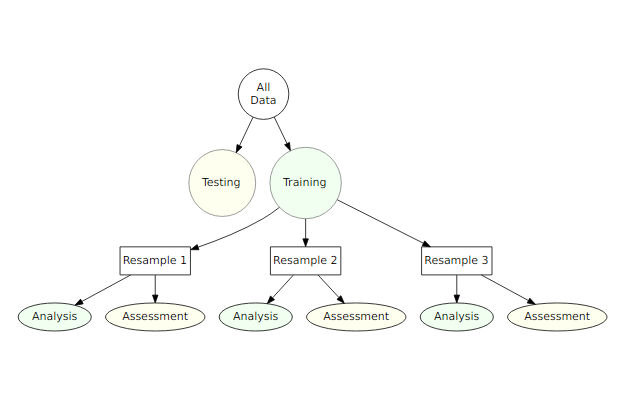
A typical scheme for splitting the data when developing a predictive model is to create an initial split of the data into a training and test set.
Then resampling is often done on subests of the training set.
In rsample, the term analysis set is used for subsets of the resampled training set; the assessment sets are the corresponding hold-out sets used to compute performance.
\(~\)
\(~\)
Grid Search is common practiace in resampling:
- Create a tuning grid of tuning parameters s
- Apply combinations of tuning parameters on the grid tuning grid with resampling.
- Each time, the assessment data are used to estimate performance metrics that maybe pooled to tune model performance
\(~\)
Nested resampling does an additional layer of resampling that separates the tuning activities from the process used to estimate the efficacy of the model:
- An outer resampling scheme is used and, for every split in the outer resample, another full set of resampling splits are created on the original analysis set.
- Once the tuning results are complete, a model is fit to each of the outer resampling splits using the best parameter associated with that resample.
- The average of the outer method’s assessment sets are a unbiased estimate of the model.
-
For example: To attempt to tune a hyper-parameter with 10 levels, we use a 10-fold cross-validation is used on the outside, and 5-fold cross-validation on the inside. Then:
- The parameter tuning will be conducted 10 times and the best parameters are determined from the average of the 5 assessment sets.
- This process occurs 10 times.
- In total, 500 models would be fit.
\(~\)
\(~\)
26.2.1 Get Started
We will use this example to tune the tree hyper-parameter from the randomForest function in the radomForest package. We will choose from a list of 12 values for which we will vary tree in seq(10, 600, 50).
We will use the follow for our nested resampling strategy:
- OUTER: A twice-repeated 5-fold cross validation will be used as the outer resampling method; it will be used to generate estimates of the overall performance.
- INNER: To tune the model, we will use estimates from each of the values of the tuning parameter from the 3 bootstrap iterations.
\(~\)
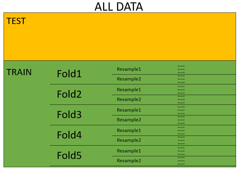
\(~\)
This means that for each of the 12 values that tree can take on in seq(10, 600, 50) we will have 5 * 2 * 3 = 30 models to be fit.
So, in total we will fit 5 * 2 * 3 * 12 = 360 models!
\(~\)
\(~\)
26.3 Create nested_cv object
Create the tibble with the resampling specifications:
TRAIN.nested_cv <- nested_cv(TRAIN,
                             outside = vfold_cv(v = 5, repeats = 2),
                             inside = bootstraps(times = 3))
TRAIN.nested_cv
# Nested resampling:
# outer: 5-fold cross-validation repeated 2 times
# inner: Bootstrap sampling
# A tibble: 10 × 4
splits id id2 inner_resamples
<list> <chr> <chr> <list>
1 <split [900/225]> Repeat1 Fold1 <boot [3 × 2]>
2 <split [900/225]> Repeat1 Fold2 <boot [3 × 2]>
3 <split [900/225]> Repeat1 Fold3 <boot [3 × 2]>
4 <split [900/225]> Repeat1 Fold4 <boot [3 × 2]>
5 <split [900/225]> Repeat1 Fold5 <boot [3 × 2]>
6 <split [900/225]> Repeat2 Fold1 <boot [3 × 2]>
7 <split [900/225]> Repeat2 Fold2 <boot [3 × 2]>
8 <split [900/225]> Repeat2 Fold3 <boot [3 × 2]>
9 <split [900/225]> Repeat2 Fold4 <boot [3 × 2]>
10 <split [900/225]> Repeat2 Fold5 <boot [3 × 2]> str(TRAIN.nested_cv,1)nest_cv [10 × 4] (S3: nested_cv/vfold_cv/rset/tbl_df/tbl/data.frame)
- attr(*, "v")= num 5
- attr(*, "repeats")= num 2
- attr(*, "breaks")= num 4
- attr(*, "pool")= num 0.1
- attr(*, "fingerprint")= chr "f039727a2aed6bda912104e921559e5c"
- attr(*, "outside")= language vfold_cv(v = 5, repeats = 2)
- attr(*, "inside")= language bootstraps(times = 3)\(~\)
\(~\)
\(~\)
We can access all of the resamples of data:
TRAIN.nested_cv$inner_resamples[[1]]
# Bootstrap sampling
# A tibble: 3 × 2
splits id
<list> <chr>
1 <split [900/326]> Bootstrap1
2 <split [900/320]> Bootstrap2
3 <split [900/346]> Bootstrap3
[[2]]
# Bootstrap sampling
# A tibble: 3 × 2
splits id
<list> <chr>
1 <split [900/324]> Bootstrap1
2 <split [900/343]> Bootstrap2
3 <split [900/352]> Bootstrap3
[[3]]
# Bootstrap sampling
# A tibble: 3 × 2
splits id
<list> <chr>
1 <split [900/339]> Bootstrap1
2 <split [900/325]> Bootstrap2
3 <split [900/318]> Bootstrap3
[[4]]
# Bootstrap sampling
# A tibble: 3 × 2
splits id
<list> <chr>
1 <split [900/321]> Bootstrap1
2 <split [900/340]> Bootstrap2
3 <split [900/319]> Bootstrap3
[[5]]
# Bootstrap sampling
# A tibble: 3 × 2
  splits            id
  <list>            <chr>
1 <split [900/340]> Bootstrap1
2 <split [900/323]> Bootstrap2
3 <split [900/335]> Bootstrap3
[[6]]
# Bootstrap sampling
# A tibble: 3 × 2
splits id
<list> <chr>
1 <split [900/333]> Bootstrap1
2 <split [900/336]> Bootstrap2
3 <split [900/333]> Bootstrap3
[[7]]
# Bootstrap sampling
# A tibble: 3 × 2
splits id
<list> <chr>
1 <split [900/322]> Bootstrap1
2 <split [900/328]> Bootstrap2
3 <split [900/317]> Bootstrap3
[[8]]
# Bootstrap sampling
# A tibble: 3 × 2
splits id
<list> <chr>
1 <split [900/329]> Bootstrap1
2 <split [900/335]> Bootstrap2
3 <split [900/319]> Bootstrap3
[[9]]
# Bootstrap sampling
# A tibble: 3 × 2
splits id
<list> <chr>
1 <split [900/327]> Bootstrap1
2 <split [900/336]> Bootstrap2
3 <split [900/337]> Bootstrap3
[[10]]
# Bootstrap sampling
# A tibble: 3 × 2
splits id
<list> <chr>
1 <split [900/351]> Bootstrap1
2 <split [900/326]> Bootstrap2
3 <split [900/330]> Bootstrap3\(~\)
\(~\)
\(~\)
We can also access individual samples or data sets used for training or assessment:
TRAIN.nested_cv$inner_resamples[[5]]# Bootstrap sampling
# A tibble: 3 × 2
splits id
<list> <chr>
1 <split [900/340]> Bootstrap1
2 <split [900/323]> Bootstrap2
3 <split [900/335]> Bootstrap3TRAIN.nested_cv$inner_resamples[[5]]$splits[[2]]<Analysis/Assess/Total>
<900/323/900>Rows: 900
Columns: 10
$ seqn <dbl> 85990, 87964, 86528, 85304, 86146, 86284, 87506, 86817, 86360…
$ riagendr <fct> Female, Male, Female, Male, Male, Male, Male, Male, Male, Fem…
$ ridageyr <dbl> 50, 21, 37, 68, 40, 46, 48, 60, 50, 42, 80, 43, 48, 31, 37, 6…
$ ridreth1 <fct> Non-Hispanic White, MexicanAmerican, Non-Hispanic Black, Non-…
$ dmdeduc2 <fct> Some college or AA degrees, Some college or AA degrees, Some …
$ dmdmartl <fct> Married, Never married, Never married, Married, Married, Marr…
$ indhhin2 <fct> "$100,000+", "$15,000-$19,999", "$45,000-$54,999", "$25,000-$…
$ bmxbmi <dbl> 33.6, 28.0, 23.9, 27.0, 26.5, 29.2, 27.7, 30.4, 41.2, 34.5, 2…
$ diq010 <fct> No Diabetes, No Diabetes, No Diabetes, No Diabetes, No Diabet…
$ lbxglu <dbl> 87, 86, 90, 91, 101, 79, 94, 119, 116, 100, 92, 111, 94, 103,…glimpse( assessment( TRAIN.nested_cv$inner_resamples[[5]]$splits[[2]] ) ) # used to assessRows: 323
Columns: 10
$ seqn <dbl> 84424, 84443, 84627, 84685, 85192, 85363, 85471, 85521, 85928…
$ riagendr <fct> Male, Male, Male, Female, Female, Female, Male, Female, Male,…
$ ridageyr <dbl> 69, 64, 80, 27, 53, 66, 63, 71, 66, 38, 55, 80, 80, 72, 37, 7…
$ ridreth1 <fct> Non-Hispanic White, Other, MexicanAmerican, Non-Hispanic Whit…
$ dmdeduc2 <fct> College grad or above, Some college or AA degrees, Less than …
$ dmdmartl <fct> Divorced, Married, Married, Married, Living with partner, Mar…
$ indhhin2 <fct> "$25,000-$34,999", "$25,000-$34,999", "$10,000-$14,999", "$45…
$ bmxbmi <dbl> 33.5, 33.8, 29.1, 25.4, 22.5, 23.2, 21.7, 31.7, 29.3, 37.5, 3…
$ diq010 <fct> Diabetes, Diabetes, Diabetes, Diabetes, Diabetes, Diabetes, D…
$ lbxglu <dbl> 429, 134, 125, 100, 122, 238, 156, 147, 154, 87, 311, 125, 19…\(~\)
\(~\)
\(~\)
\(~\)
\(~\)
\(~\)
26.4 Function mapping with purrr
We will frequently make use of map functions within the purrr library.
\(~\)
\(~\)
\(~\)
\(~\)
\(~\)
\(~\)
26.5 Helper Functions
\(~\)
The majority of the work is done by using a sequence of helper-functions and purrr mappers.
We know our goal is to work with the inner_resamples of our TRAIN.nested_cv tibble.
Given a cut of data, and tuning parameters n_tree = seq(10, 600, 50) we will write a function to estimate F1:
\(~\)
\(~\)
26.5.1 F1_Tree Helper Function
Here we can borrow from what we already know about a predicting and scoring models along with some helper functions.
We want the first input of our function to be a cut of data, an object from our rsplit::nested_cv function to the TRAIN.nested_cv tibble and our second to be a value of ’ntree`:
This function will:
- take: a cut of data and tuning-parameter
- train a model with: a value of tuning-parameter and the corresponding training set
- score the corresponding testing data
- return the estimate for the f1 metric
f1_tree <- function(object, my_tree = 761) {  # my_tree = 761

  model_rf <- randomForest::randomForest(diq010 ~ riagendr + ridageyr + ridreth1 + dmdeduc2 + dmdmartl + indhhin2 + bmxbmi + lbxglu,
                       data = analysis(object),
                       ntree = my_tree,
                       mtry = 7)

  holdout_pred_class <- predict(model_rf, assessment(object), "class")

  dt <- tibble::as_tibble(cbind(assessment(object), holdout_pred_class))

  yd_f1 <- yardstick::f_meas(data=dt, truth=diq010, holdout_pred_class)

  F1_Score <- yd_f1$.estimate

  return(F1_Score)
}

# test the function
f1_tree(TRAIN.nested_cv$inner_resamples[[5]]$splits[[3]])
[1] 0.6666667\(~\)
\(~\)
26.5.2 F1_Tree_Wrapper Function
If you understood the last function, this one is even easier. This function will allow us to reverse the call order of f1_tree:
f1_tree_wrapper <- function(my_tree , object){ f1_tree(object, my_tree) }

f1_tree_wrapper( 123, TRAIN.nested_cv$inner_resamples[[5]]$splits[[3]] )
[1] 0.68\(~\)
\(~\)
26.5.3 Tune_Over_Trees Function
We will develop the function that will allow us to tune over ntree.
Again, this function’s input expects a sample of data as it’s input.
Given a sample of data, for each value of the tuning parameter, we want to make an assessment:
tune_over_trees <- function(object) {
  tune_over_trees_results <- tibble( my_tree =  seq(10, 600, 50) )  # sample(10:600, size=15, replace=FALSE)

  tune_over_trees_results$F1_Score <- map_dbl(tune_over_trees_results$my_tree,
                                             f1_tree_wrapper,
                                             object = object)
  tune_over_trees_results
}

# test the function
tune_over_trees( TRAIN.nested_cv$inner_resamples[[1]]$splits[[2]] )
# A tibble: 12 × 2
my_tree F1_Score
<dbl> <dbl>
1 10 0.595
2 60 0.619
3 110 0.602
4 160 0.619
5 210 0.602
6 260 0.602
7 310 0.602
8 360 0.585
9 410 0.585
10 460 0.585
11 510 0.602
12 560 0.585\(~\)
\(~\)
26.5.4 Summarise_Tune_Results Function
This function will be used to summarise our results from the inner nest into the outer nest.
This function will again take an inner object from rsample::nested_cv
-
map_dfmaps the sample data to thetune_over_treesfunction which is already waiting for it; and an inner assessment is made. - Return the row-bound tibble
map_df(object$splits, tune_over_trees)is our result from that has 3 bootstrap results - Next we group the assessments by the value of
ntreewe perform a summary step. * Compute the count, max, median, and min of the F1_Score from the inner bootstrap estimate.- Since we have only have 3 bootstraps, the returning max, median, and min values will completely contain all the estimates from the inner nest, so we can pool them into the Outer Layer.
We can’t test this function for a slice of data, as it’s intedended to be used with another function:
summarize_tune_results( TRAIN.nested_cv$inner_resamples[[1]]$splits[[2]] )Error in `group_by()`:
! Must group by variables found in `.data`.
✖ Column `my_tree` is not found.#### Summary below\(~\)
\(~\)
We conclude this Section with an Index of Functions we defined:
26.5.5 Helper Function Quick Refrence
A Quick Reference to The Helper Functions
26.5.5.1 F1 Tree Helper Function
f1_tree <- function(object, my_tree = 761) {  # my_tree = 761

  model_rf <- randomForest::randomForest(diq010 ~ riagendr + ridageyr + ridreth1 + dmdeduc2 + dmdmartl + indhhin2 + bmxbmi + lbxglu,
                       data = analysis(object),
                       ntree = my_tree,
                       mtry = 7)

  holdout_pred_class <- predict(model_rf, assessment(object), "class")

  dt <- tibble::as_tibble(cbind(assessment(object), holdout_pred_class))

  yd_f1 <- yardstick::f_meas(data=dt, truth=diq010, holdout_pred_class)

  F1_Score <- yd_f1$.estimate

  return(F1_Score)
}
26.5.5.2 F1 Tree Wrapper Function
f1_tree_wrapper <- function(my_tree , object){ f1_tree(object, my_tree) }26.5.5.3 Tune Over Trees
26.5.5.4 Summarise Tune Results Function
\(~\)
\(~\)
\(~\)
\(~\)
\(~\)
26.6 Run Inner Nest
Now to run the inner nest!
Time difference of 49.38535 secs\(~\)
\(~\)
26.6.1 Inner Nest Results
List of 10
 $ : tibble [12 × 5] (S3: tbl_df/tbl/data.frame)
  ..$ my_tree        : num [1:12] 10 60 110 160 210 260 310 360 410 460 ...
  ..$ max_F1_Score   : num [1:12] 0.608 0.619 0.605 0.619 0.585 ...
  ..$ median_F1_Score: num [1:12] 0.6 0.595 0.585 0.603 0.583 ...
  ..$ min_F1_Score   : num [1:12] 0.553 0.564 0.575 0.571 0.579 ...
  ..$ n              : int [1:12] 3 3 3 3 3 3 3 3 3 3 ...
 $ : tibble [12 × 5] (S3: tbl_df/tbl/data.frame)
  ..$ my_tree        : num [1:12] 10 60 110 160 210 260 310 360 410 460 ...
  ..$ max_F1_Score   : num [1:12] 0.606 0.629 0.636 0.634 0.62 ...
  ..$ median_F1_Score: num [1:12] 0.596 0.609 0.634 0.617 0.605 ...
  ..$ min_F1_Score   : num [1:12] 0.594 0.583 0.593 0.605 0.593 ...
  ..$ n              : int [1:12] 3 3 3 3 3 3 3 3 3 3 ...
 $ : tibble [12 × 5] (S3: tbl_df/tbl/data.frame)
  ..$ my_tree        : num [1:12] 10 60 110 160 210 260 310 360 410 460 ...
  ..$ max_F1_Score   : num [1:12] 0.706 0.641 0.653 0.653 0.653 ...
  ..$ median_F1_Score: num [1:12] 0.604 0.633 0.642 0.625 0.642 ...
  ..$ min_F1_Score   : num [1:12] 0.586 0.583 0.577 0.589 0.583 ...
  ..$ n              : int [1:12] 3 3 3 3 3 3 3 3 3 3 ...
 $ : tibble [12 × 5] (S3: tbl_df/tbl/data.frame)
  ..$ my_tree        : num [1:12] 10 60 110 160 210 260 310 360 410 460 ...
  ..$ max_F1_Score   : num [1:12] 0.593 0.659 0.654 0.636 0.641 ...
  ..$ median_F1_Score: num [1:12] 0.582 0.627 0.615 0.621 0.628 ...
  ..$ min_F1_Score   : num [1:12] 0.571 0.608 0.614 0.615 0.623 ...
  ..$ n              : int [1:12] 3 3 3 3 3 3 3 3 3 3 ...
 $ : tibble [12 × 5] (S3: tbl_df/tbl/data.frame)
  ..$ my_tree        : num [1:12] 10 60 110 160 210 260 310 360 410 460 ...
  ..$ max_F1_Score   : num [1:12] 0.66 0.66 0.647 0.66 0.66 ...
  ..$ median_F1_Score: num [1:12] 0.587 0.58 0.6 0.611 0.58 ...
  ..$ min_F1_Score   : num [1:12] 0.529 0.492 0.523 0.523 0.5 ...
  ..$ n              : int [1:12] 3 3 3 3 3 3 3 3 3 3 ...
 $ : tibble [12 × 5] (S3: tbl_df/tbl/data.frame)
  ..$ my_tree        : num [1:12] 10 60 110 160 210 260 310 360 410 460 ...
  ..$ max_F1_Score   : num [1:12] 0.617 0.617 0.59 0.597 0.633 ...
  ..$ median_F1_Score: num [1:12] 0.56 0.587 0.587 0.589 0.596 ...
  ..$ min_F1_Score   : num [1:12] 0.55 0.574 0.556 0.566 0.561 ...
  ..$ n              : int [1:12] 3 3 3 3 3 3 3 3 3 3 ...
 $ : tibble [12 × 5] (S3: tbl_df/tbl/data.frame)
  ..$ my_tree        : num [1:12] 10 60 110 160 210 260 310 360 410 460 ...
  ..$ max_F1_Score   : num [1:12] 0.583 0.636 0.659 0.66 0.674 ...
  ..$ median_F1_Score: num [1:12] 0.548 0.609 0.587 0.579 0.579 ...
  ..$ min_F1_Score   : num [1:12] 0.484 0.575 0.543 0.571 0.571 ...
  ..$ n              : int [1:12] 3 3 3 3 3 3 3 3 3 3 ...
 $ : tibble [12 × 5] (S3: tbl_df/tbl/data.frame)
  ..$ my_tree        : num [1:12] 10 60 110 160 210 260 310 360 410 460 ...
  ..$ max_F1_Score   : num [1:12] 0.639 0.685 0.667 0.685 0.667 ...
  ..$ median_F1_Score: num [1:12] 0.63 0.675 0.667 0.675 0.658 ...
  ..$ min_F1_Score   : num [1:12] 0.587 0.627 0.636 0.657 0.657 ...
  ..$ n              : int [1:12] 3 3 3 3 3 3 3 3 3 3 ...
 $ : tibble [12 × 5] (S3: tbl_df/tbl/data.frame)
  ..$ my_tree        : num [1:12] 10 60 110 160 210 260 310 360 410 460 ...
  ..$ max_F1_Score   : num [1:12] 0.634 0.659 0.675 0.644 0.649 ...
  ..$ median_F1_Score: num [1:12] 0.598 0.608 0.651 0.641 0.644 ...
  ..$ min_F1_Score   : num [1:12] 0.541 0.578 0.561 0.568 0.602 ...
  ..$ n              : int [1:12] 3 3 3 3 3 3 3 3 3 3 ...
 $ : tibble [12 × 5] (S3: tbl_df/tbl/data.frame)
  ..$ my_tree        : num [1:12] 10 60 110 160 210 260 310 360 410 460 ...
  ..$ max_F1_Score   : num [1:12] 0.688 0.687 0.659 0.667 0.68 ...
  ..$ median_F1_Score: num [1:12] 0.646 0.636 0.646 0.611 0.667 ...
  ..$ min_F1_Score   : num [1:12] 0.523 0.541 0.548 0.548 0.548 ...
..$ n : int [1:12] 3 3 3 3 3 3 3 3 3 3 ...NULLtuning_results[[1]]# A tibble: 12 × 5
my_tree max_F1_Score median_F1_Score min_F1_Score n
<dbl> <dbl> <dbl> <dbl> <int>
1 10 0.608 0.6 0.553 3
2 60 0.619 0.595 0.564 3
3 110 0.605 0.585 0.575 3
4 160 0.619 0.603 0.571 3
5 210 0.585 0.583 0.579 3
6 260 0.622 0.587 0.585 3
7 310 0.603 0.587 0.585 3
8 360 0.605 0.602 0.571 3
9 410 0.593 0.587 0.583 3
10 460 0.602 0.592 0.587 3
11 510 0.595 0.585 0.571 3
12 560 0.595 0.585 0.583 3tuning_results[[6]]# A tibble: 12 × 5
my_tree max_F1_Score median_F1_Score min_F1_Score n
<dbl> <dbl> <dbl> <dbl> <int>
1 10 0.617 0.56 0.550 3
2 60 0.617 0.587 0.574 3
3 110 0.590 0.587 0.556 3
4 160 0.597 0.589 0.566 3
5 210 0.633 0.596 0.561 3
6 260 0.633 0.593 0.574 3
7 310 0.608 0.581 0.561 3
8 360 0.633 0.587 0.574 3
9 410 0.615 0.604 0.587 3
10 460 0.615 0.589 0.547 3
11 510 0.615 0.574 0.527 3
12 560 0.623 0.549 0.547 3label_nested_cv <- TRAIN.nested_cv %>%
mutate(RowNumber = row_number()) %>%
select(RowNumber,id,id2)
label_nested_cv# A tibble: 10 × 3
RowNumber id id2
<int> <chr> <chr>
1 1 Repeat1 Fold1
2 2 Repeat1 Fold2
3 3 Repeat1 Fold3
4 4 Repeat1 Fold4
5 5 Repeat1 Fold5
6 6 Repeat2 Fold1
7 7 Repeat2 Fold2
8 8 Repeat2 Fold3
9 9 Repeat2 Fold4
10 10 Repeat2 Fold5 my_tree max_F1_Score median_F1_Score min_F1_Score n id id2
1 10 0.6075949 0.6000000 0.5526316 3 Repeat1 Fold1
2 60 0.6190476 0.5945946 0.5641026 3 Repeat1 Fold1
3 110 0.6052632 0.5853659 0.5753425 3 Repeat1 Fold1
4 160 0.6190476 0.6027397 0.5714286 3 Repeat1 Fold1
5 210 0.5853659 0.5833333 0.5789474 3 Repeat1 Fold1
6 260 0.6216216 0.5866667 0.5853659 3 Repeat1 Fold1
7 310 0.6027397 0.5866667 0.5853659 3 Repeat1 Fold1
8 360 0.6052632 0.6024096 0.5714286 3 Repeat1 Fold1
9 410 0.5925926 0.5866667 0.5833333 3 Repeat1 Fold1
10 460 0.6024096 0.5915493 0.5866667 3 Repeat1 Fold1
11 510 0.5945946 0.5853659 0.5714286 3 Repeat1 Fold1
12 560 0.5945946 0.5853659 0.5833333 3 Repeat1 Fold1
Attaching package: 'scales'The following object is masked from 'package:purrr':
discardThe following object is masked from 'package:readr':
col_factor'data.frame': 120 obs. of 7 variables:
$ my_tree : num 10 60 110 160 210 260 310 360 410 460 ...
$ max_F1_Score : num 0.608 0.619 0.605 0.619 0.585 ...
$ median_F1_Score: num 0.6 0.595 0.585 0.603 0.583 ...
$ min_F1_Score : num 0.553 0.564 0.575 0.571 0.579 ...
$ n : int 3 3 3 3 3 3 3 3 3 3 ...
$ id : chr "Repeat1" "Repeat1" "Repeat1" "Repeat1" ...
$ id2 : chr "Fold1" "Fold1" "Fold1" "Fold1" ...\(~\)
\(~\)
\(~\)
\(~\)
26.6.2 Inner Nest Results Graphs
Check out the Facet - Fold tab below:
26.6.2.1 Facet - Fold
ggplot(pooled_inner, aes(x = my_tree , y = median_F1_Score, shape = id, color = id )) +
  geom_point(aes(size = median_F1_Score)) +
  geom_line() +
  facet_wrap(.~id2)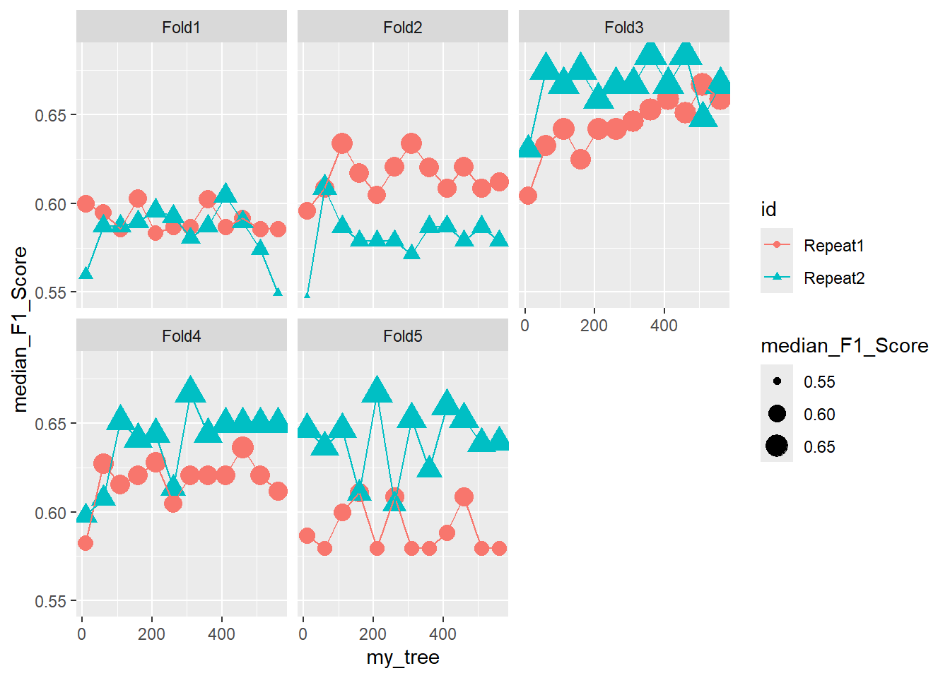
26.6.2.2 Facet - Fold with Errors
ggplot(pooled_inner, aes(x = my_tree , y = median_F1_Score, shape = id, color = id )) +
  geom_line() +
  geom_errorbar(aes(ymin=min_F1_Score, ymax=max_F1_Score)) +
  facet_wrap(.~id2)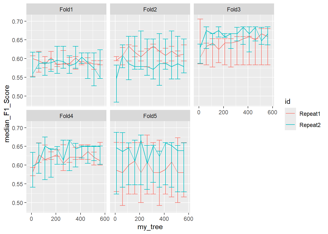
26.6.2.3 Facet - Repeat
ggplot(pooled_inner, aes(x = my_tree , y = median_F1_Score, shape = id2, color = id2 )) +
  geom_point(aes(size = median_F1_Score)) +
  geom_line() +
  facet_wrap(.~id)
26.6.2.4 Unorganized
ggplot(pooled_inner, aes(x = my_tree , y = median_F1_Score, shape = id2, color = id )) +
  geom_point(aes(size = median_F1_Score)) +
geom_line() 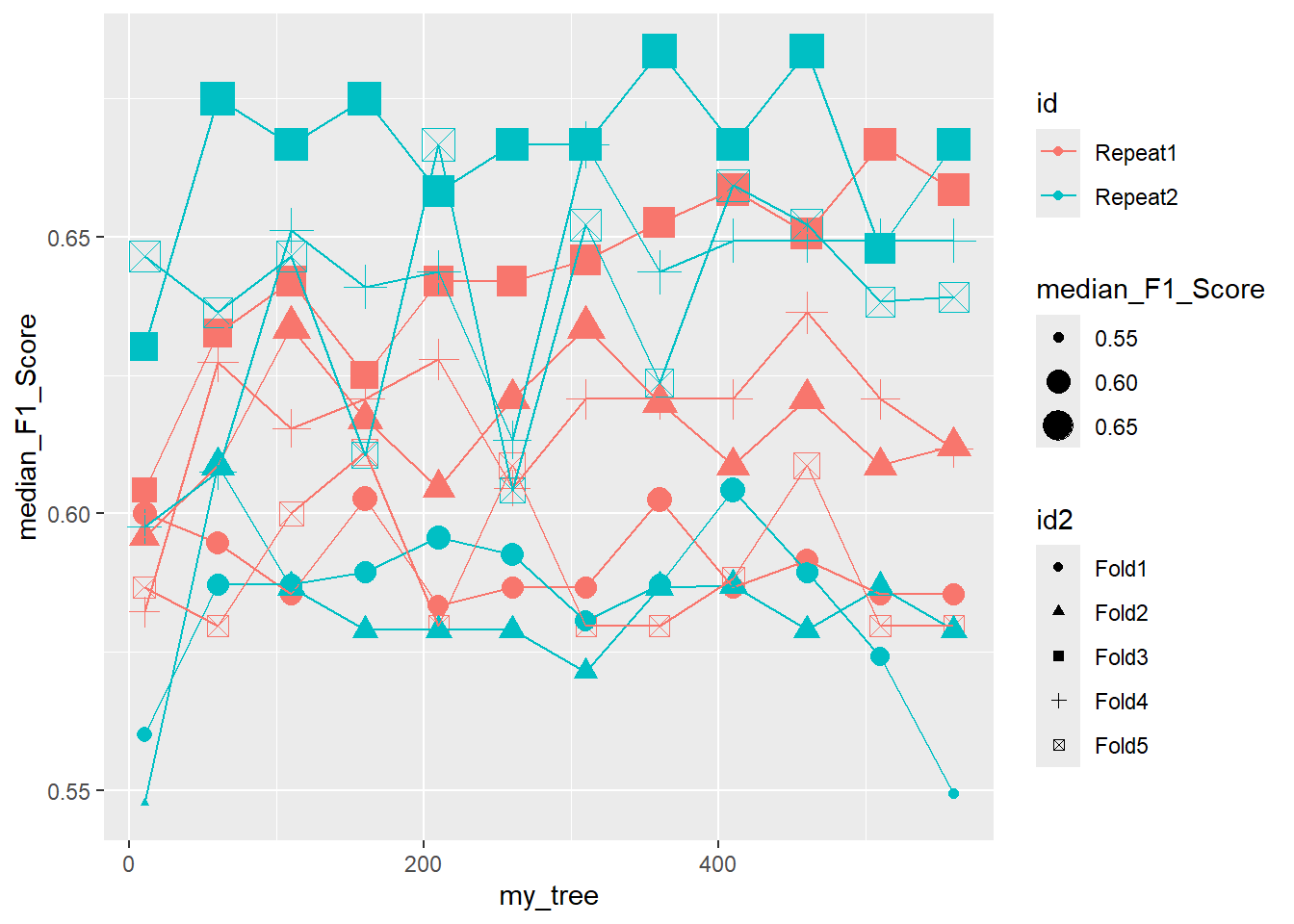
26.7
#{.unnumbered}
\(~\)
\(~\)
\(~\)
\(~\)
\(~\)
26.8 Max Best F1 Value Function
We will use this helper function to select the corresponding row of data that contains the max_F1_Score from our summary in pooled_inner.
max_BEST_F1 <- function(data) { data[ which.max(data$max_F1_Score) , ] }


# test the function
tuning_results[[10]]
# A tibble: 12 × 5
my_tree max_F1_Score median_F1_Score min_F1_Score n
<dbl> <dbl> <dbl> <dbl> <int>
1 10 0.688 0.646 0.523 3
2 60 0.687 0.636 0.541 3
3 110 0.659 0.646 0.548 3
4 160 0.667 0.611 0.548 3
5 210 0.68 0.667 0.548 3
6 260 0.652 0.604 0.535 3
7 310 0.653 0.652 0.554 3
8 360 0.637 0.624 0.541 3
9 410 0.660 0.659 0.548 3
10 460 0.66 0.652 0.541 3
11 510 0.652 0.638 0.529 3
12 560 0.659 0.639 0.529 3max_BEST_F1(tuning_results[[10]])# A tibble: 1 × 5
my_tree max_F1_Score median_F1_Score min_F1_Score n
<dbl> <dbl> <dbl> <dbl> <int>
1 10 0.688 0.646 0.523 3\(~\)
\(~\)
\(~\)
\(~\)
\(~\)
\(~\)
26.9 Running Outer Nest From Inner Pooled
We will find the values of ntree that had the highest performing F1 by sample, we will map those and an outer split of the sample to f1_tree to obtain our outer-inner estimates.
# A tibble: 10 × 5
   my_tree max_F1_Score median_F1_Score min_F1_Score     n
     <dbl>        <dbl>           <dbl>        <dbl> <int>
 1     260        0.622           0.587        0.585     3
 2     310        0.638           0.634        0.629     3
 3      10        0.706           0.604        0.586     3
 4     310        0.667           0.621        0.608     3
 5     260        0.68            0.609        0.523     3
 6     210        0.633           0.596        0.561     3
 7     210        0.674           0.579        0.571     3
 8      60        0.685           0.675        0.627     3
 9     110        0.675           0.651        0.561     3
10 10 0.688 0.646 0.523 3Rows: 10
Columns: 5
$ splits <list> [<vfold_split[900 x 225 x 1125 x 10]>], [<vfold_split…
$ id <chr> "Repeat1", "Repeat1", "Repeat1", "Repeat1", "Repeat1",…
$ id2 <chr> "Fold1", "Fold2", "Fold3", "Fold4", "Fold5", "Fold1", …
$ inner_resamples <list> [<bootstraps[3 x 2]>], [<bootstraps[3 x 2]>], [<boots…
$ my_tree <dbl> 260, 310, 10, 310, 260, 210, 210, 60, 110, 10Time difference of 48.34574 secsTRAIN.nested_cv.results$F1_SCORE [1] 0.6666667 0.7878788 0.5573770 0.5098039 0.6428571 0.4897959 0.7213115
[8] 0.6666667 0.5555556 0.5769231summary(TRAIN.nested_cv.results$F1_SCORE) Min. 1st Qu. Median Mean 3rd Qu. Max.
0.4898 0.5560 0.6099 0.6175 0.6667 0.7879 TRAIN.nested_cv.results# Nested resampling:
# outer: 5-fold cross-validation repeated 2 times
# inner: Bootstrap sampling
# A tibble: 10 × 6
splits id id2 inner_resamples my_tree F1_SCORE
<list> <chr> <chr> <list> <dbl> <dbl>
1 <split [900/225]> Repeat1 Fold1 <boot [3 × 2]> 260 0.667
2 <split [900/225]> Repeat1 Fold2 <boot [3 × 2]> 310 0.788
3 <split [900/225]> Repeat1 Fold3 <boot [3 × 2]> 10 0.557
4 <split [900/225]> Repeat1 Fold4 <boot [3 × 2]> 310 0.510
5 <split [900/225]> Repeat1 Fold5 <boot [3 × 2]> 260 0.643
6 <split [900/225]> Repeat2 Fold1 <boot [3 × 2]> 210 0.490
7 <split [900/225]> Repeat2 Fold2 <boot [3 × 2]> 210 0.721
8 <split [900/225]> Repeat2 Fold3 <boot [3 × 2]> 60 0.667
9 <split [900/225]> Repeat2 Fold4 <boot [3 × 2]> 110 0.556
10 <split [900/225]> Repeat2 Fold5 <boot [3 × 2]> 10 0.577\(~\)
\(~\)
\(~\)
\(~\)
\(~\)
\(~\)
26.10 Run Outer Nest
Time difference of 21.70855 secsdiff.outer - diff.innerTime difference of -27.6768 secsouter_only[[1]]
# A tibble: 12 × 2
my_tree F1_Score
<dbl> <dbl>
1 10 0.623
2 60 0.635
3 110 0.688
4 160 0.667
5 210 0.688
6 260 0.667
7 310 0.667
8 360 0.667
9 410 0.667
10 460 0.667
11 510 0.688
12 560 0.688
[[2]]
# A tibble: 12 × 2
my_tree F1_Score
<dbl> <dbl>
1 10 0.645
2 60 0.725
3 110 0.716
4 160 0.783
5 210 0.746
6 260 0.776
7 310 0.776
8 360 0.758
9 410 0.765
10 460 0.765
11 510 0.746
12 560 0.746
[[3]]
# A tibble: 12 × 2
my_tree F1_Score
<dbl> <dbl>
1 10 0.491
2 60 0.538
3 110 0.52
4 160 0.531
5 210 0.52
6 260 0.510
7 310 0.522
8 360 0.538
9 410 0.510
10 460 0.52
11 510 0.549
12 560 0.52
[[4]]
# A tibble: 12 × 2
my_tree F1_Score
<dbl> <dbl>
1 10 0.519
2 60 0.510
3 110 0.510
4 160 0.566
5 210 0.538
6 260 0.510
7 310 0.538
8 360 0.510
9 410 0.510
10 460 0.538
11 510 0.538
12 560 0.538
[[5]]
# A tibble: 12 × 2
my_tree F1_Score
<dbl> <dbl>
1 10 0.667
2 60 0.655
3 110 0.655
4 160 0.655
5 210 0.630
6 260 0.655
7 310 0.655
8 360 0.655
9 410 0.655
10 460 0.655
11 510 0.655
12 560 0.655
[[6]]
# A tibble: 12 × 2
my_tree F1_Score
<dbl> <dbl>
1 10 0.642
2 60 0.538
3 110 0.56
4 160 0.52
5 210 0.588
6 260 0.577
7 310 0.571
8 360 0.56
9 410 0.6
10 460 0.549
11 510 0.588
12 560 0.588
[[7]]
# A tibble: 12 × 2
my_tree F1_Score
<dbl> <dbl>
1 10 0.698
2 60 0.721
3 110 0.721
4 160 0.746
5 210 0.733
6 260 0.733
7 310 0.746
8 360 0.733
9 410 0.721
10 460 0.733
11 510 0.721
12 560 0.733
[[8]]
# A tibble: 12 × 2
my_tree F1_Score
<dbl> <dbl>
1 10 0.609
2 60 0.676
3 110 0.667
4 160 0.667
5 210 0.676
6 260 0.667
7 310 0.676
8 360 0.696
9 410 0.676
10 460 0.667
11 510 0.676
12 560 0.657
[[9]]
# A tibble: 12 × 2
my_tree F1_Score
<dbl> <dbl>
1 10 0.542
2 60 0.536
3 110 0.571
4 160 0.536
5 210 0.509
6 260 0.509
7 310 0.582
8 360 0.536
9 410 0.545
10 460 0.556
11 510 0.536
12 560 0.571
[[10]]
# A tibble: 12 × 2
my_tree F1_Score
<dbl> <dbl>
1 10 0.5
2 60 0.679
3 110 0.571
4 160 0.679
5 210 0.6
6 260 0.654
7 310 0.571
8 360 0.56
9 410 0.627
10 460 0.6
11 510 0.627
12 560 0.627str(outer_only,1)List of 10
$ : tibble [12 × 2] (S3: tbl_df/tbl/data.frame)
$ : tibble [12 × 2] (S3: tbl_df/tbl/data.frame)
$ : tibble [12 × 2] (S3: tbl_df/tbl/data.frame)
$ : tibble [12 × 2] (S3: tbl_df/tbl/data.frame)
$ : tibble [12 × 2] (S3: tbl_df/tbl/data.frame)
$ : tibble [12 × 2] (S3: tbl_df/tbl/data.frame)
$ : tibble [12 × 2] (S3: tbl_df/tbl/data.frame)
$ : tibble [12 × 2] (S3: tbl_df/tbl/data.frame)
$ : tibble [12 × 2] (S3: tbl_df/tbl/data.frame)
$ : tibble [12 × 2] (S3: tbl_df/tbl/data.frame)outer_only_2 <- NULL
for (i in 1:length(outer_only)){
outer_only_2[[i]] <- cbind( outer_only[[i]], label_nested_cv[i, c('id','id2')] )
}
outer_only_3 <- outer_only_2 %>% bind_rows()
outer_summary <- outer_only_3 %>%
group_by(id,id2, my_tree) %>%
summarize(outer_F1_Score = mean(F1_Score),
n = length(F1_Score)) %>%
ungroup()`summarise()` has regrouped the output.
ℹ Summaries were computed grouped by id, id2, and my_tree.
ℹ Output is grouped by id and id2.
ℹ Use `summarise(.groups = "drop_last")` to silence this message.
ℹ Use `summarise(.by = c(id, id2, my_tree))` for per-operation grouping
(`?dplyr::dplyr_by`) instead.outer_summary# A tibble: 120 × 5
id id2 my_tree outer_F1_Score n
<chr> <chr> <dbl> <dbl> <int>
1 Repeat1 Fold1 10 0.623 1
2 Repeat1 Fold1 60 0.635 1
3 Repeat1 Fold1 110 0.688 1
4 Repeat1 Fold1 160 0.667 1
5 Repeat1 Fold1 210 0.688 1
6 Repeat1 Fold1 260 0.667 1
7 Repeat1 Fold1 310 0.667 1
8 Repeat1 Fold1 360 0.667 1
9 Repeat1 Fold1 410 0.667 1
10 Repeat1 Fold1 460 0.667 1
# ℹ 110 more rows\(~\)
\(~\)
26.10.1 Outer Nest Summary Graphs
Some output summary graphs:
26.10.1.1 Facet - Fold
ggplot(outer_summary, aes(x=my_tree, y=outer_F1_Score, color = id , shape = id  ) ) +
  geom_point(aes(size = outer_F1_Score)) +
  geom_line()  +
  facet_wrap(.~id2)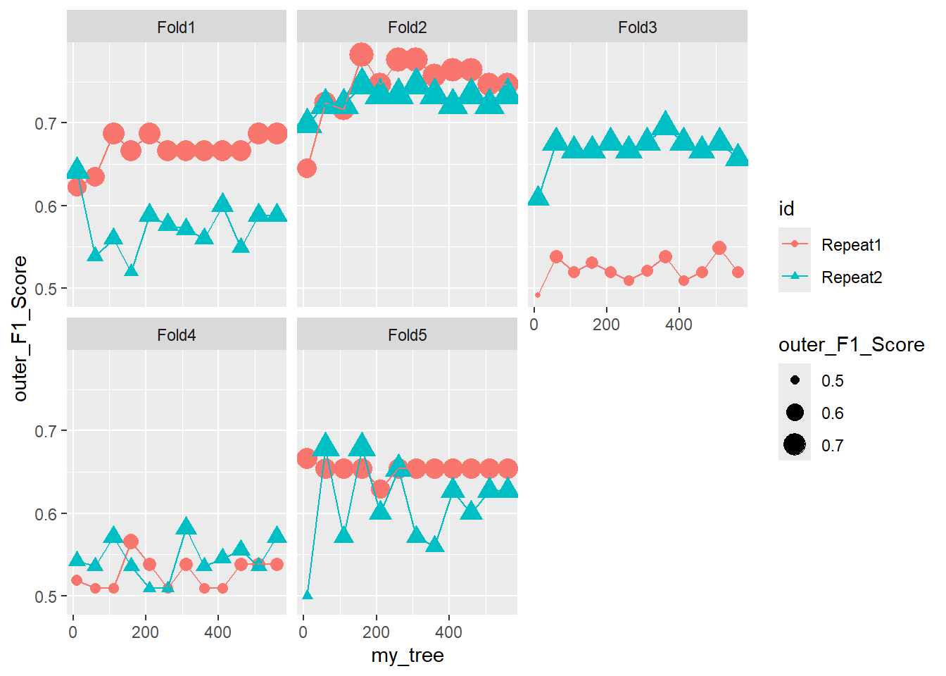
26.10.1.2 Unorganized
ggplot(outer_summary, aes(x=my_tree, y=outer_F1_Score, color = id , shape = id2  ) ) +
  geom_point(aes(size = outer_F1_Score)) +
  geom_line()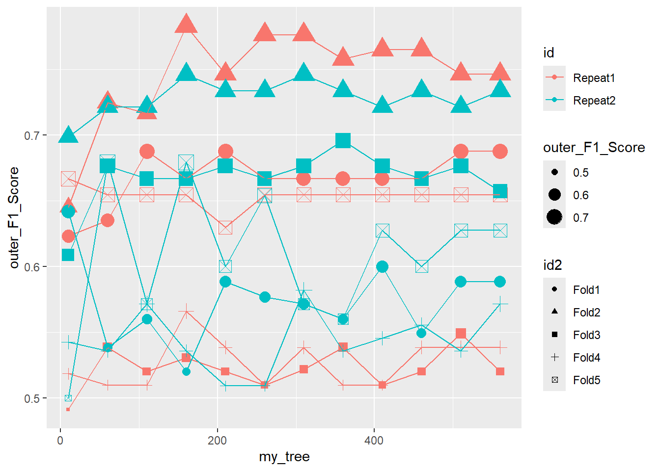
26.10.1.3 Facet - Repeat
ggplot(outer_summary, aes(x=my_tree, y=outer_F1_Score, color = id2 , shape = id2  ) ) +
  geom_point(aes(size = outer_F1_Score)) +
  geom_line()  +
  facet_wrap(.~id)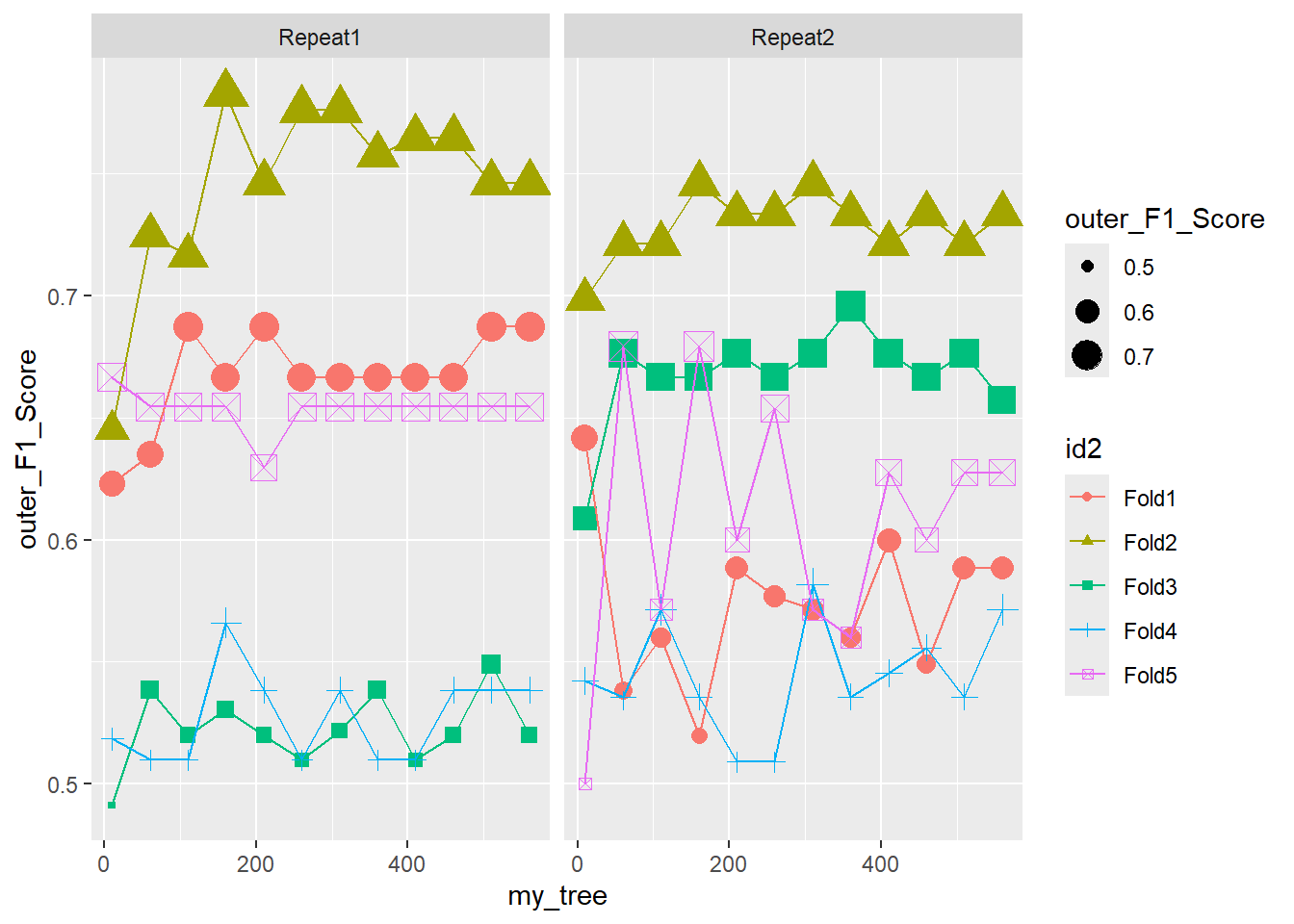
\(~\)
\(~\)
\(~\)
\(~\)
\(~\)
\(~\)
26.11 Inner V Outer
Pooled_Inner_L <- pooled_inner %>%
  select(id2, id, my_tree, max_F1_Score, median_F1_Score, min_F1_Score) %>%
  gather(max_F1_Score, median_F1_Score, min_F1_Score, key='Inner_F1_Scores', value=Inner_F1_Score) %>%
  mutate(Inner_Type = ifelse( Inner_F1_Scores == 'max_F1_Score', "MAX",
                      ifelse( Inner_F1_Scores == 'median_F1_Score', "MED",
                      ifelse( Inner_F1_Scores == 'min_F1_Score', "MIN", "NA" ) )  ) ) %>%
  select(-Inner_F1_Scores)


Outer_Summary <- outer_summary %>%
  select(id2, id, my_tree, outer_F1_Score)

inner_v_outer <- Pooled_Inner_L %>%
  left_join(Outer_Summary, by=c('id','id2','my_tree')) %>%
  select(id2, id, Inner_Type, my_tree, Inner_F1_Score, outer_F1_Score) %>%
  arrange(id2, id, Inner_Type, my_tree, Inner_F1_Score, outer_F1_Score)

glimpse(inner_v_outer)
Rows: 360
Columns: 6
$ id2 <chr> "Fold1", "Fold1", "Fold1", "Fold1", "Fold1", "Fold1", "…
$ id <chr> "Repeat1", "Repeat1", "Repeat1", "Repeat1", "Repeat1", …
$ Inner_Type <chr> "MAX", "MAX", "MAX", "MAX", "MAX", "MAX", "MAX", "MAX",…
$ my_tree <dbl> 10, 60, 110, 160, 210, 260, 310, 360, 410, 460, 510, 56…
$ Inner_F1_Score <dbl> 0.6075949, 0.6190476, 0.6052632, 0.6190476, 0.5853659, …
$ outer_F1_Score <dbl> 0.6229508, 0.6349206, 0.6875000, 0.6666667, 0.6875000, …Rows: 360
Columns: 5
Groups: id2, id, Inner_Type [30]
$ id2 <chr> "Fold1", "Fold1", "Fold1", "Fold1", "Fold1", "Fold1", "Fold…
$ id <chr> "Repeat1", "Repeat1", "Repeat1", "Repeat1", "Repeat1", "Rep…
$ Inner_Type <chr> "MAX", "MAX", "MAX", "MAX", "MAX", "MAX", "MAX", "MAX", "MA…
$ my_tree <dbl> 10, 60, 110, 160, 210, 260, 310, 360, 410, 460, 510, 560, 1…
$ n <int> 1, 1, 1, 1, 1, 1, 1, 1, 1, 1, 1, 1, 1, 1, 1, 1, 1, 1, 1, 1,…\(~\)
\(~\)
26.11.1 Inner V Outer Summary Graphs
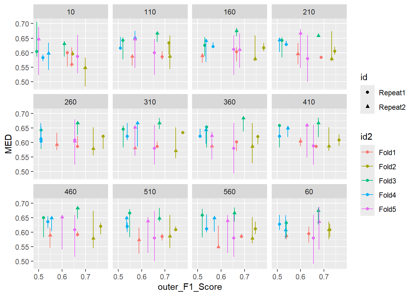
26.11.1.1 Facet - my_tree
inner_min_max_v_outer <- inner_v_outer %>%
         mutate( my_tree_char = as.character(my_tree) ) %>%
         mutate( Fold_Sample = paste0(id2,'_',id)) %>%
         spread( key=Inner_Type, Inner_F1_Score)

ggplot(inner_min_max_v_outer , aes(x = outer_F1_Score , y = MED, shape = id , color = id2 )) +
  geom_point( ) +
  geom_line( ) +
  geom_errorbar(aes(ymin=MIN, ymax=MAX)) +
  facet_wrap(.~ my_tree_char )
`geom_line()`: Each group consists of only one observation.
ℹ Do you need to adjust the group aesthetic?
`geom_line()`: Each group consists of only one observation.
ℹ Do you need to adjust the group aesthetic?
`geom_line()`: Each group consists of only one observation.
ℹ Do you need to adjust the group aesthetic?
`geom_line()`: Each group consists of only one observation.
ℹ Do you need to adjust the group aesthetic?
`geom_line()`: Each group consists of only one observation.
ℹ Do you need to adjust the group aesthetic?
`geom_line()`: Each group consists of only one observation.
ℹ Do you need to adjust the group aesthetic?
`geom_line()`: Each group consists of only one observation.
ℹ Do you need to adjust the group aesthetic?
`geom_line()`: Each group consists of only one observation.
ℹ Do you need to adjust the group aesthetic?
`geom_line()`: Each group consists of only one observation.
ℹ Do you need to adjust the group aesthetic?
`geom_line()`: Each group consists of only one observation.
ℹ Do you need to adjust the group aesthetic?
`geom_line()`: Each group consists of only one observation.
ℹ Do you need to adjust the group aesthetic?
`geom_line()`: Each group consists of only one observation.
ℹ Do you need to adjust the group aesthetic?