Diabetes date/time-stamped data shall be analyzed using the random forest method. The DIABETES data sets are provided for use in 1994 AI in Medicine symposium submissions (AIM-94 data set provided by Michael Kahn, MD, PhD, Washington University, St. Louis, MO) and may be downloaded from https://archive.ics.uci.edu/ml/datasets/Diabetes. The DIABETES data contain:
Data-Codes: a listing of the codes used in the data sets.
Domain-Description: This file describes the basic physiology and patho-physiology of diabetes mellitus and its treatment.
data-[01-70]: data sets covering several weeks’ to months’ worth of outpatient care on 70 patients.
Source: Michael Kahn, MD, PhD, Washington University, St. Louis, MO
Data Set Information: Diabetes patient records were obtained from two sources: an automatic electronic recording device and paper records. The automatic device had an internal clock to timestamp events, whereas the paper records only provided “logical time” slots (breakfast, lunch, dinner, bedtime). For paper records, fixed times were assigned to breakfast (08:00), lunch (12:00), dinner (18:00), and bedtime (22:00). Thus paper records have fictitious uniform recording times whereas electronic records have more realistic time stamps.
Diabetes files consist of four fields per record. Each field is separated by a tab and each record is separated by a newline.
File format:
Date in MM-DD-YYYY format
Time in XX:YY format
Code
Value
The Code field is deciphered as follows:
33 = Regular insulin dose
34 = NPH insulin dose
35 = UltraLente insulin dose
48 = Unspecified blood glucose measurement
57 = Unspecified blood glucose measurement
58 = Pre-breakfast blood glucose measurement
59 = Post-breakfast blood glucose measurement
60 = Pre-lunch blood glucose measurement
61 = Post-lunch blood glucose measurement
62 = Pre-supper blood glucose measurement
63 = Post-supper blood glucose measurement
64 = Pre-snack blood glucose measurement
65 = Hypoglycemic symptoms
66 = Typical meal ingestion
67 = More-than-usual meal ingestion
68 = Less-than-usual meal ingestion
69 = Typical exercise activity
70 = More-than-usual exercise activity
71 = Less-than-usual exercise activity
72 = Unspecified special event
11 Download Data
Our first task is to use R to download the data.
The code below creates a temporary directory within the current project directory, downloads a compressed file from a URL to that temporary directory, and then extracts the contents of the compressed file into the same temporary directory.
Code
temp_path<-"Temp_DM_Path"#This line creates a new directory with the path specified by file.path(here::here(),temp_path). The here::here() function returns the path to the current project directory, and file.path combines this with the value of temp_path to create the full path to the new temporary directory.dir.create(file.path(here::here(),temp_path))my_tar_file<-file.path(here::here(),temp_path,'diabetes-data.tar.Z')# This line creates a variable my_url and assigns it the value of a URL that points to a compressed file.my_url<-'https://archive.ics.uci.edu/ml/machine-learning-databases/diabetes/diabetes-data.tar.Z'# This line downloads the file from the URL specified by my_url and saves it to the local path specified by my_tar_file. The mode = "wb" argument specifies that the file should be saved in binary mode.download.file(my_url, my_tar_file, mode ="wb")# This line uses the archive_extract function from the archive package to extract the contents of the compressed file specified by my_tar_file into the directory specified by dir= file.path(here::here(),temp_path), which is the same temporary directory created in step 2.archive::archive_extract(my_tar_file, dir=file.path(here::here(),temp_path))
11.1 Load Data
Our analysis begins with file path definitions followed by the read_in_text_from_file_no function used to import the diabetes data.
The goal of using purrr functions instead of for loops is to allow you to break common list manipulation challenges into independent pieces:
How can you solve the problem for a single element of the list? Once you’ve solved that problem, purrr takes care of generalizing your solution to every element in the list.
If you’re solving a complex problem, how can you break it down into bite-sized pieces that allow you to advance one small step towards a solution? With purrr, you get lots of small pieces that you can compose together with the pipe.
This structure makes it easier to solve new problems. It also makes it easier to understand your solutions to old problems when you re-read your old code.
purrr functions are implemented in C making them very fast.
Code
DM2_TIME_RAW<-purrr::map_dfr(tibble_of_file_paths$file_no, # list of columns function(x){read_in_text_from_file_no(x)})
Since we have saved the data as an RDS we can remove the temporary files:
The data are a matrix (data.frame) of 29,330 rows and 5 columns. The column names are Date (character of mm-dd-yyy), Time (character of h:mm and hh:mm), Code (character of two-digit numbers), Value (character of three-digit numbers), and file_no (number from 1 to 70). The Code number definitions are listed in the R script listing below and are referenced by the Code_Table tibble we define below.
Code
Code_Table<-tribble(~Code, ~Code_Description,33 , "Regular insulin dose",34 , "NPH insulin dose",35 , "UltraLente insulin dose",48 , "Unspecified blood glucose measurement", # This decode value is the same as 5757 , "Unspecified blood glucose measurement", # This decode value is the same as 4858 , "Pre-breakfast blood glucose measurement",59 , "Post-breakfast blood glucose measurement",60 , "Pre-lunch blood glucose measurement",61 , "Post-lunch blood glucose measurement",62 , "Pre-supper blood glucose measurement",63 , "Post-supper blood glucose measurement",64 , "Pre-snack blood glucose measurement",65 , "Hypoglycemic symptoms",66 , "Typical meal ingestion",67 , "More-than-usual meal ingestion",68 , "Less-than-usual meal ingestion",69 , "Typical exercise activity",70 , "More-than-usual exercise activity",71 , "Less-than-usual exercise activity",72 , "Unspecified special event")%>%# What does this mean? mutate(Code_Invalid =if_else(Code%in%c(48,57,72), TRUE, FALSE))%>%mutate(Code_New =if_else(Code_Invalid==TRUE, 999, Code))Code_Table
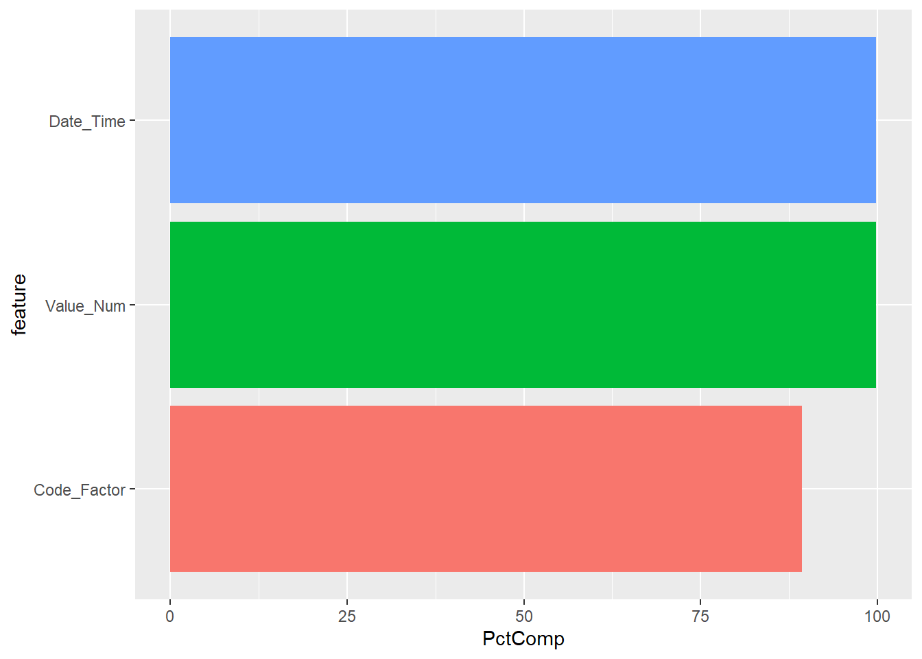
The result is the raw, imported data in DM2_TIME_RAW are conditioned, assigned to object DM2_TIME, and DM2_TIME_RAW is removed from the computing environment. The conditioning combines the dates in the Date column with the times in the Time are combined into a date time string, Date_Time_Char (mm-dd-yyyy h:mm or hh:mm), which then is converted into the date time format yyyy-mm-dd hh:mm:ss in column Date_Time. The numeric value of the character Value is assigned to column Value_Num. The character form of the codes in Code are redefined as numeric. A new column, Record_ID, is assigned the row number (1 to 29,330).
To ascertain if the complete records are indeed complete, a bar plot showing the percent complete for value number (blue), date and time (green), and code (red) is shown in Figure \(\ref{fig:Per_Complete}\). The abscissa is the percent complete from 0 to 100.
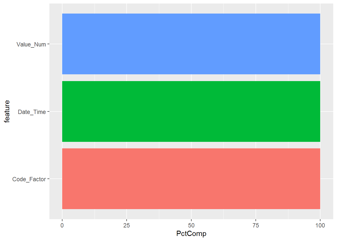
Examination of the data reveal not all records are complete. The section of code identifies these records after joining the data with the scrubbed code table data. The unknown measurement data are assigned to the Unknown_Measurements object.
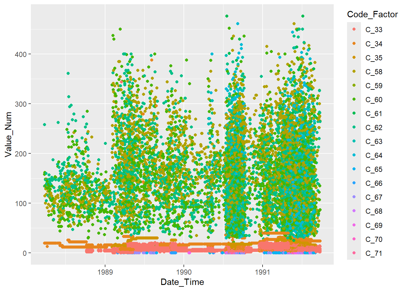
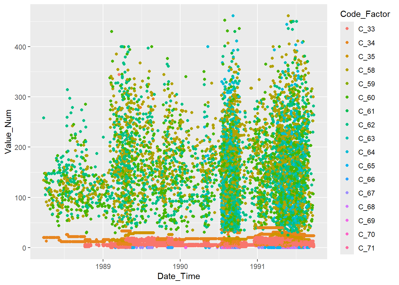
Similarly, complete records are assigned to the Known_Measurements object. The data in this object are plotted (Figure \(\ref{fig:known_measures}\)) with Value_Num on the ordinate and Date_Time (year) on the abscissa. The legend is color coded by Code.
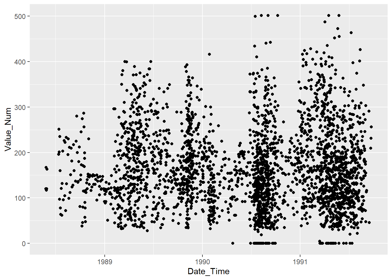
We can take a look at the UnKnown Measurements below, R will give us a warning that there are 86 which either have missing Date_Time or missing Value_Num.
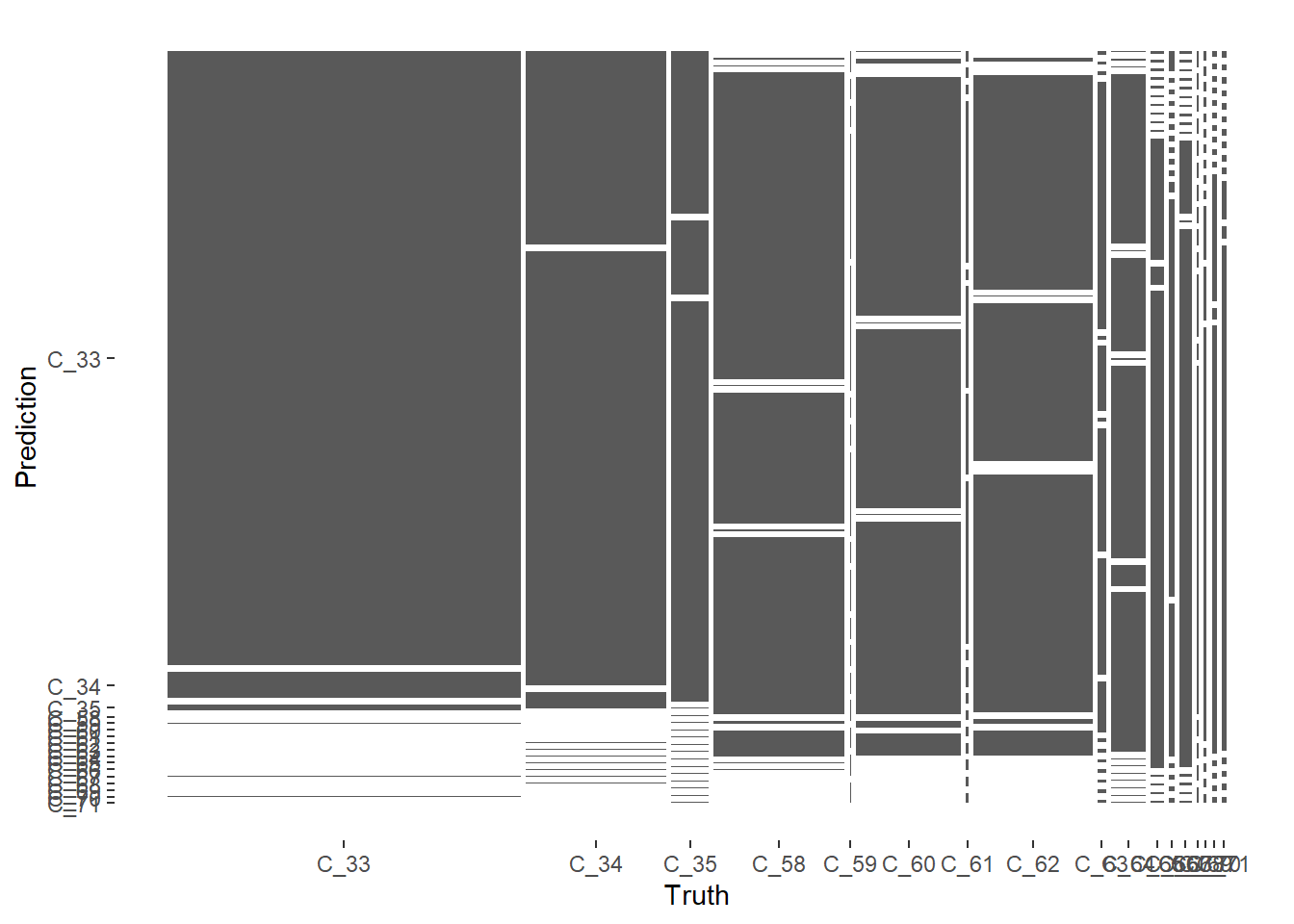
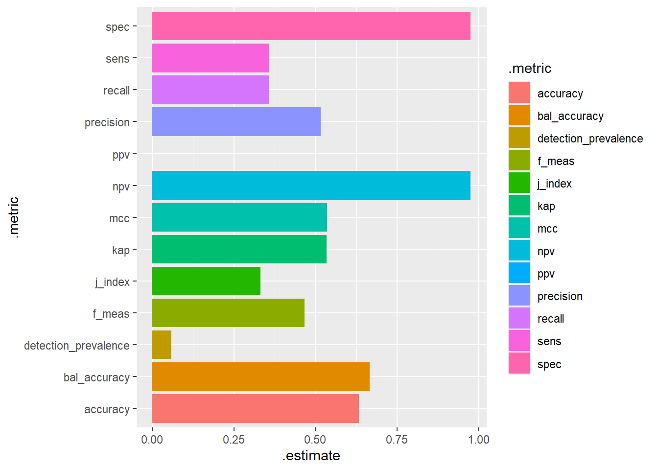
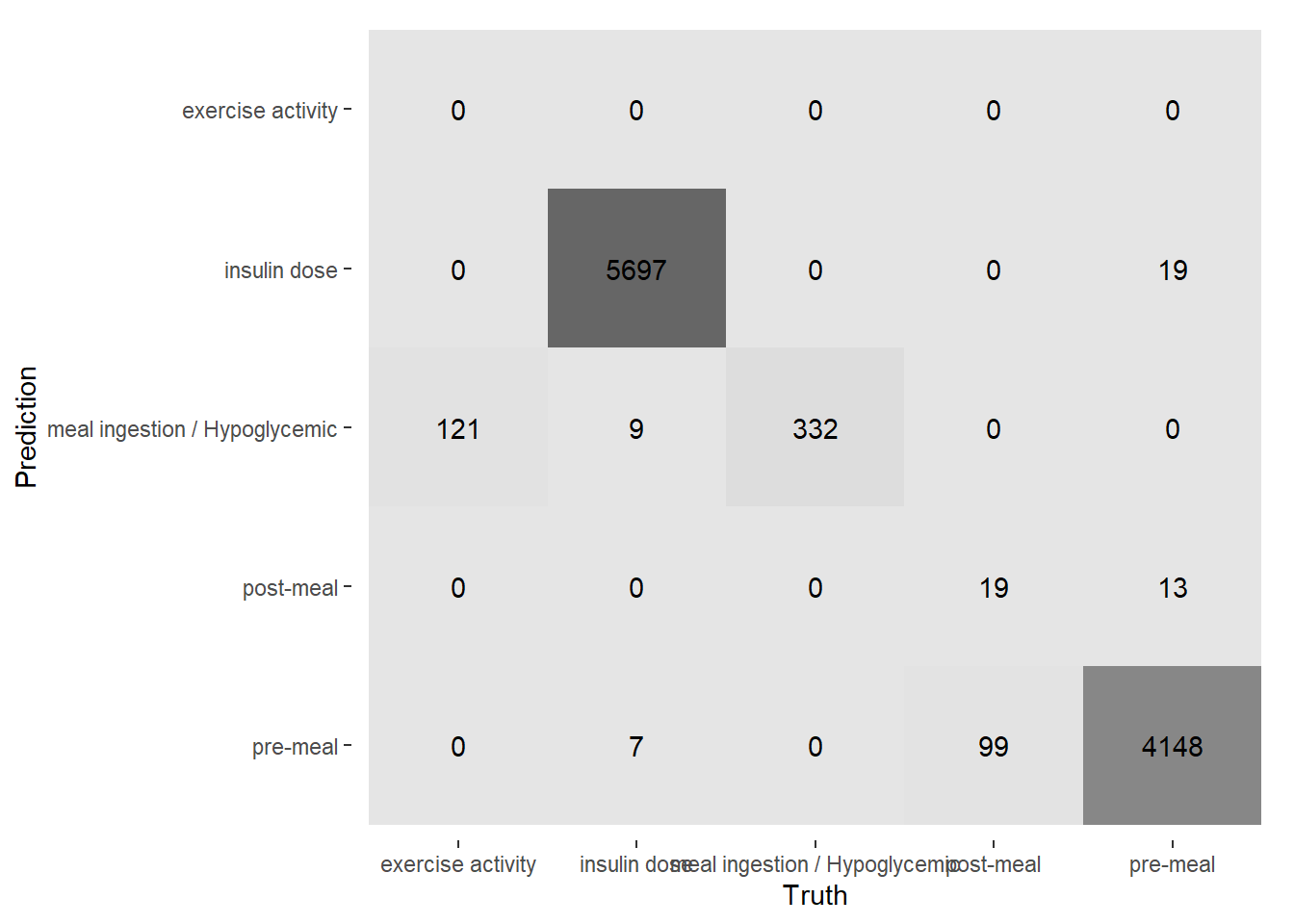
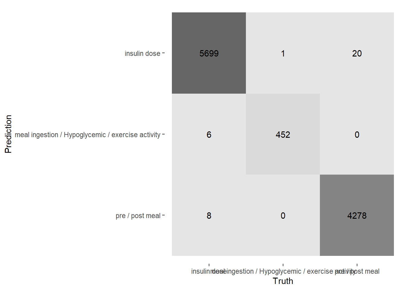
The Confusion Matrix that we see above is the confusion matrix from fitting the model against the training data so it is overly optimistic in terms of predictions.
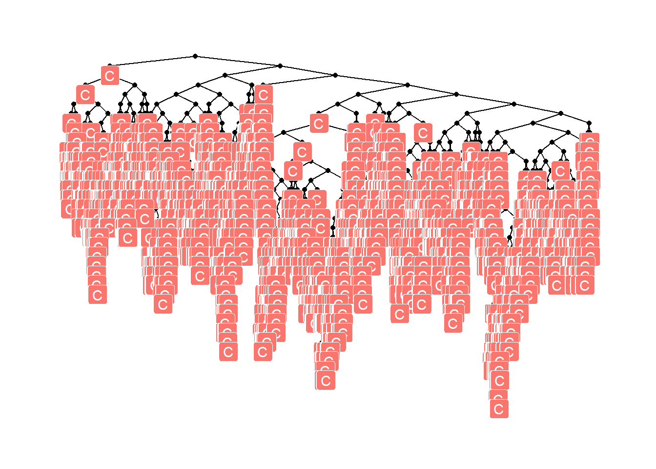
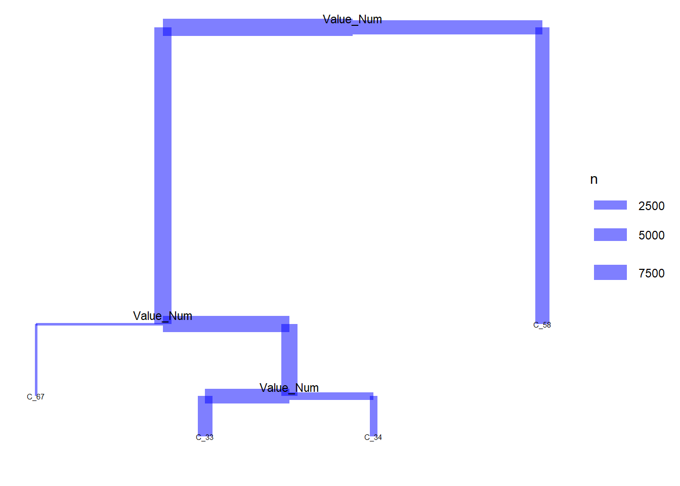
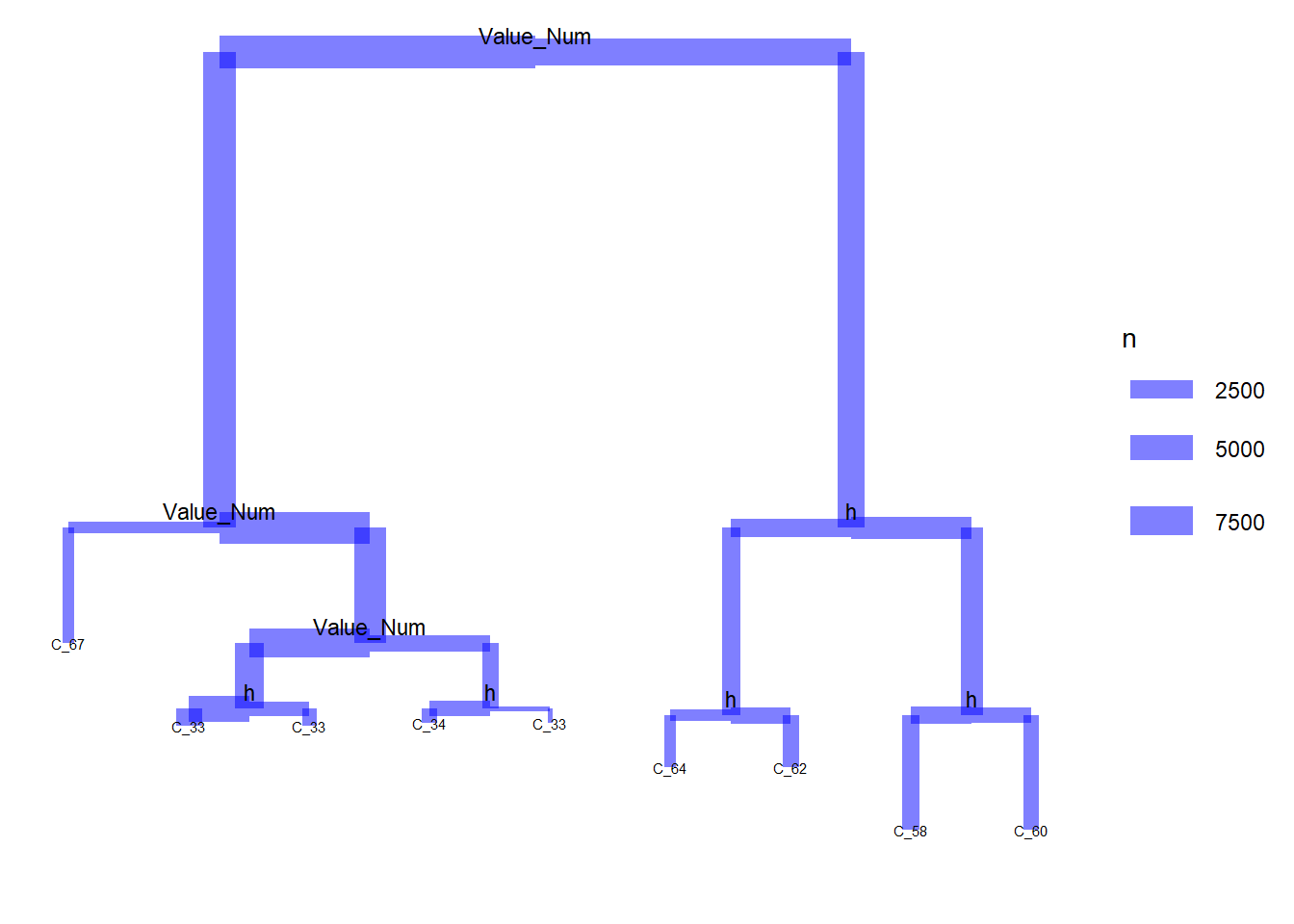
Random Forest is a collection of Decision Trees, we can look at the individual trees in the forest by using one of the two following functions.
The following objects are masked from 'package:lubridate':
%--%, union
The following objects are masked from 'package:dplyr':
as_data_frame, groups, union
The following objects are masked from 'package:purrr':
compose, simplify
The following object is masked from 'package:tidyr':
crossing
The following object is masked from 'package:tibble':
as_data_frame
The following objects are masked from 'package:stats':
decompose, spectrum
The following object is masked from 'package:base':
union
Code
plot_rf_tree<-function(final_model, tree_num, shorten_label=TRUE){# get tree by indextree<-randomForest::getTree(final_model, k =tree_num, labelVar =TRUE)%>%tibble::rownames_to_column()%>%# make leaf split points to NA, so the 0s won't get plottedmutate(`split point` =ifelse(is.na(prediction), `split point`, NA))# prepare data frame for graphgraph_frame<-data.frame(from =rep(tree$rowname, 2), to =c(tree$`left daughter`, tree$`right daughter`))# convert to graph and delete the last node that we don't want to plotgraph<-graph_from_data_frame(graph_frame)%>%delete_vertices("0")# set node labelsV(graph)$node_label<-gsub("_", " ", as.character(tree$`split var`))if(shorten_label){V(graph)$leaf_label<-substr(as.character(tree$prediction), 1, 1)}V(graph)$split<-as.character(round(tree$`split point`, digits =2))# plotplot<-ggraph(graph, 'tree')+theme_graph()+geom_edge_link()+geom_node_point()+geom_node_label(aes(label =leaf_label, fill =leaf_label), na.rm =TRUE, repel =FALSE, colour ="white", show.legend =FALSE)print(plot)}
Code
plot_rf_tree(rf_model, 456)
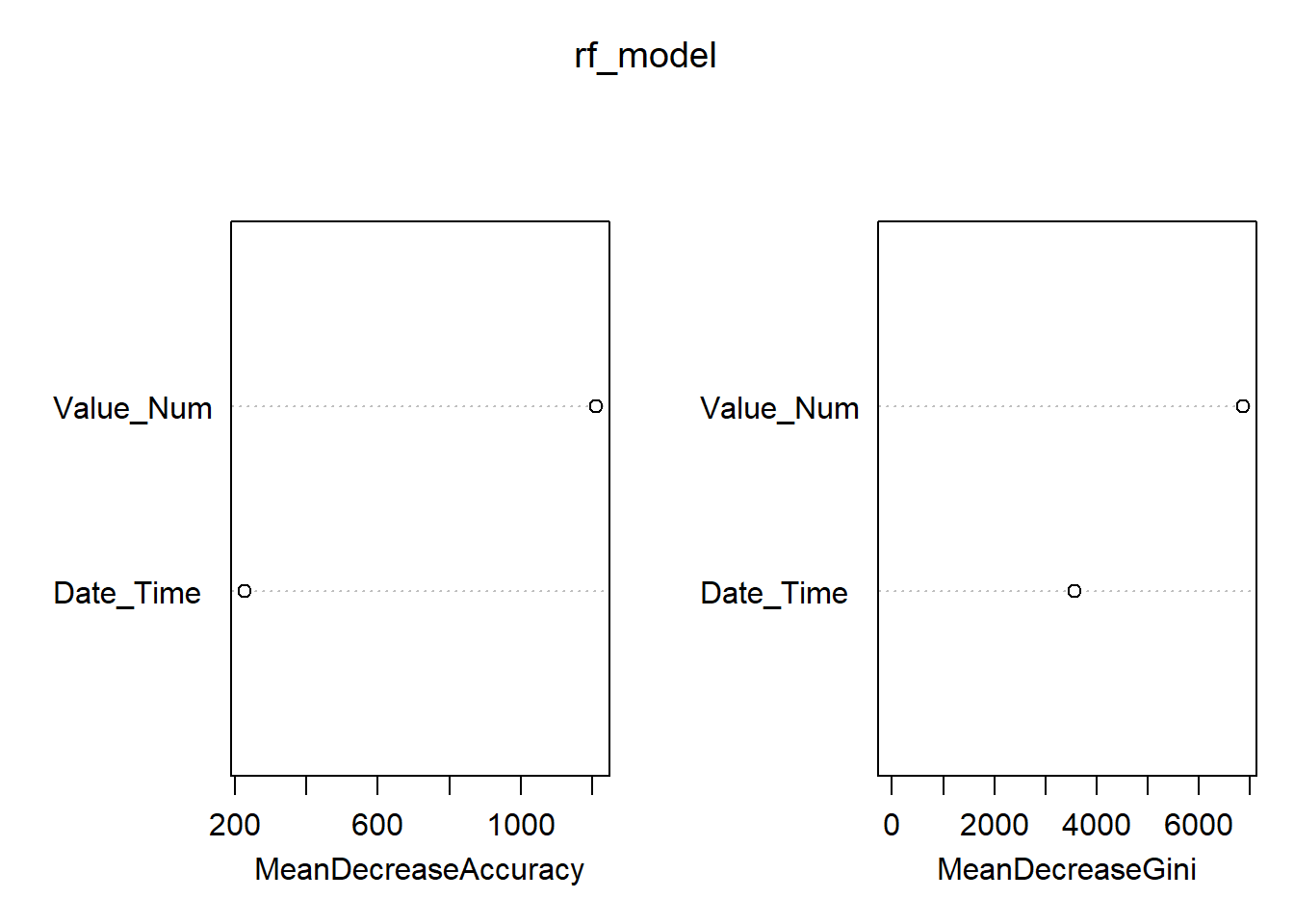
Random Forest models normally come equipped with feature importances which we can access with the varImpPlot function in this instance:
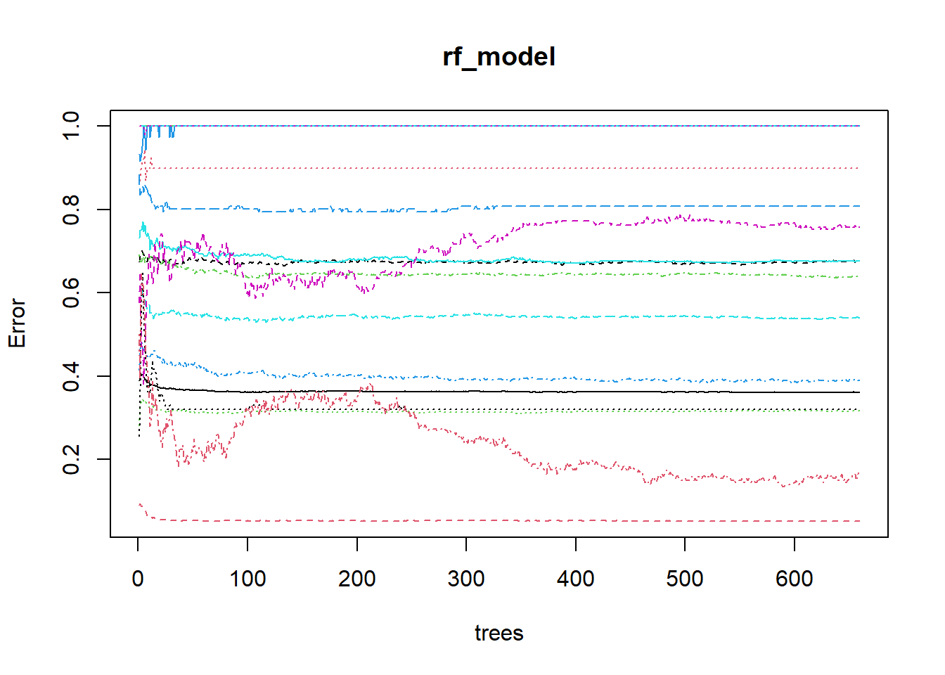
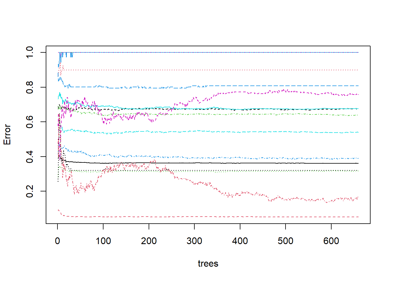
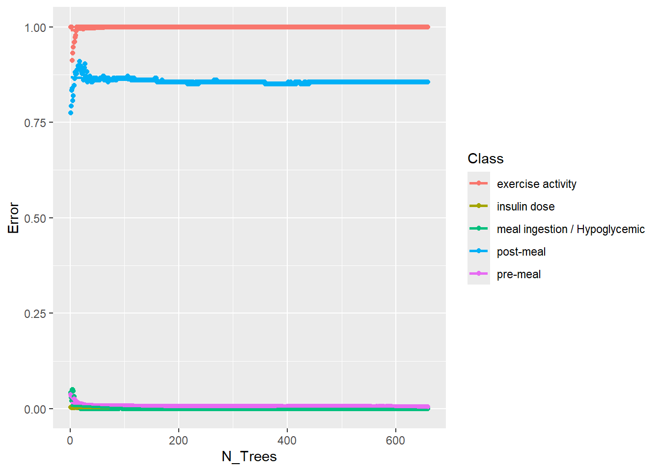
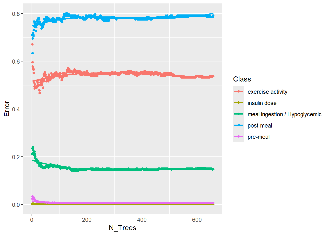
Let’s see if we can figure out what is going on with the above graph. We can extract the err.rate and ntree from the model object and place them in a matplot to match the above graph.
Code
err<-rf_model$err.rateN_trees<-1:rf_model$ntreematplot(N_trees , err, type ='l', xlab="trees", ylab="Error")
derivation of plot of randomForest model output
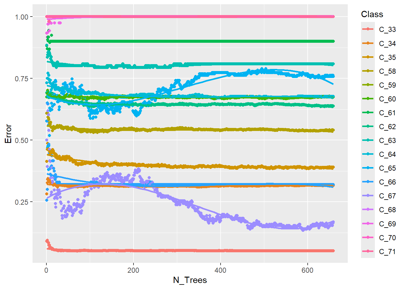
We can improve this a bit by performing the computations ourselves and keeping track of things:
Warning: While computing multiclass `precision()`, some levels had no predicted events
(i.e. `true_positive + false_positive = 0`).
Precision is undefined in this case, and those levels will be removed from the
averaged result.
Note that the following number of true events actually occurred for each
problematic event level:
'C_68': 13, 'C_69': 29, 'C_70': 49, 'C_71': 43
While computing multiclass `precision()`, some levels had no predicted events
(i.e. `true_positive + false_positive = 0`).
Precision is undefined in this case, and those levels will be removed from the
averaged result.
Note that the following number of true events actually occurred for each
problematic event level:
'C_68': 13, 'C_69': 29, 'C_70': 49, 'C_71': 43
Warning: Removed 1 row containing missing values or values outside the scale range
(`geom_bar()`).
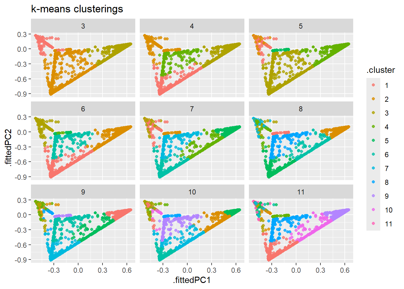
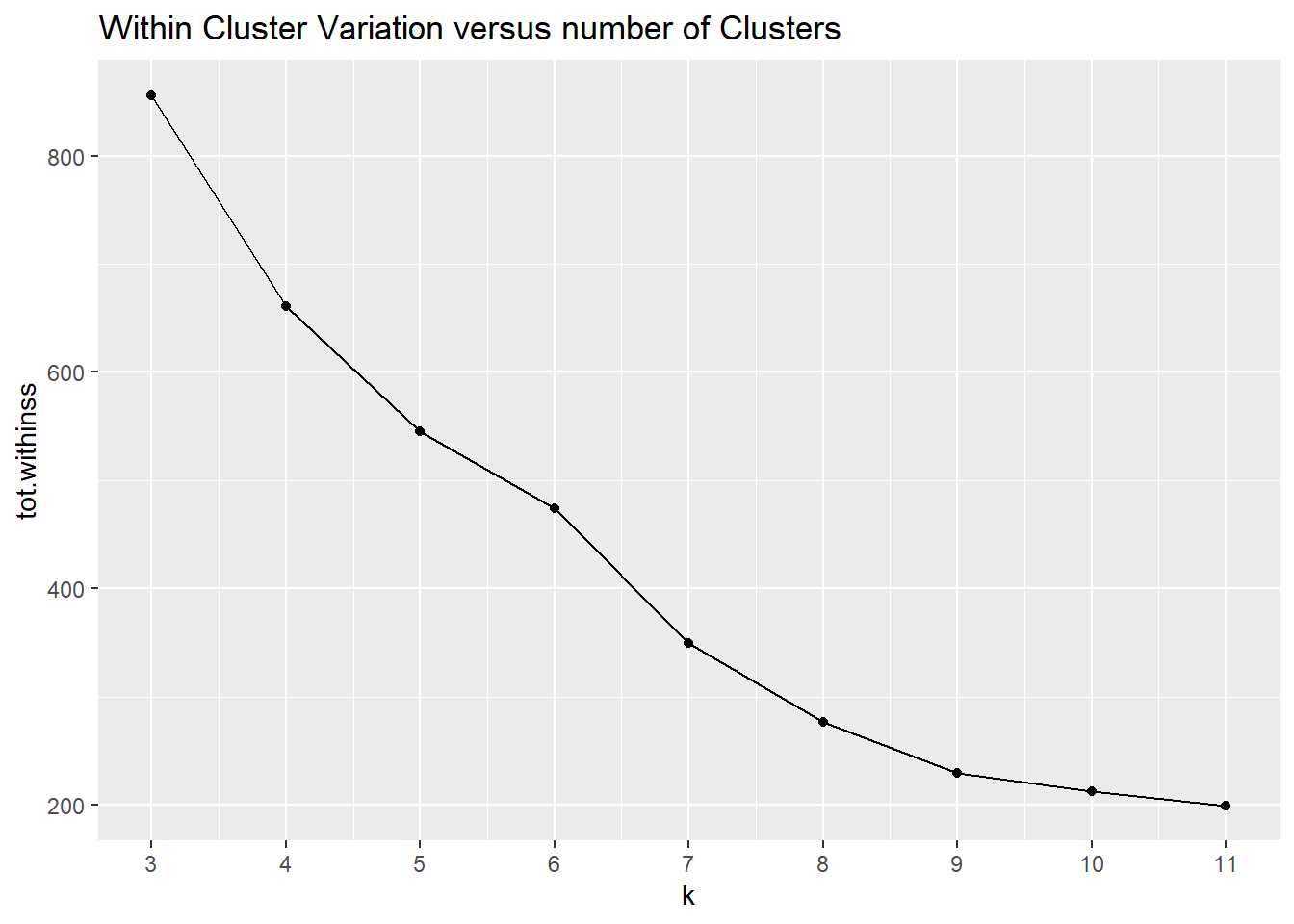
To aide us further, we will perform a k-means clustering on the probabilities to get a sense of how many classes we should have. Our first step in this endeavor will be to create a sample of roughly 60 % of the available probabilities:
Warning: While computing multiclass `precision()`, some levels had no predicted events
(i.e. `true_positive + false_positive = 0`).
Precision is undefined in this case, and those levels will be removed from the
averaged result.
Note that the following number of true events actually occurred for each
problematic event level:
'C_68': 13, 'C_69': 29, 'C_70': 49, 'C_71': 43
While computing multiclass `precision()`, some levels had no predicted events
(i.e. `true_positive + false_positive = 0`).
Precision is undefined in this case, and those levels will be removed from the
averaged result.
Note that the following number of true events actually occurred for each
problematic event level:
'C_68': 13, 'C_69': 29, 'C_70': 49, 'C_71': 43
Warning: While computing multiclass `precision()`, some levels had no predicted events
(i.e. `true_positive + false_positive = 0`).
Precision is undefined in this case, and those levels will be removed from the
averaged result.
Note that the following number of true events actually occurred for each
problematic event level:
'exercise activity': 121
Warning: Removed 86 rows containing missing values or values outside the scale range
(`geom_point()`).
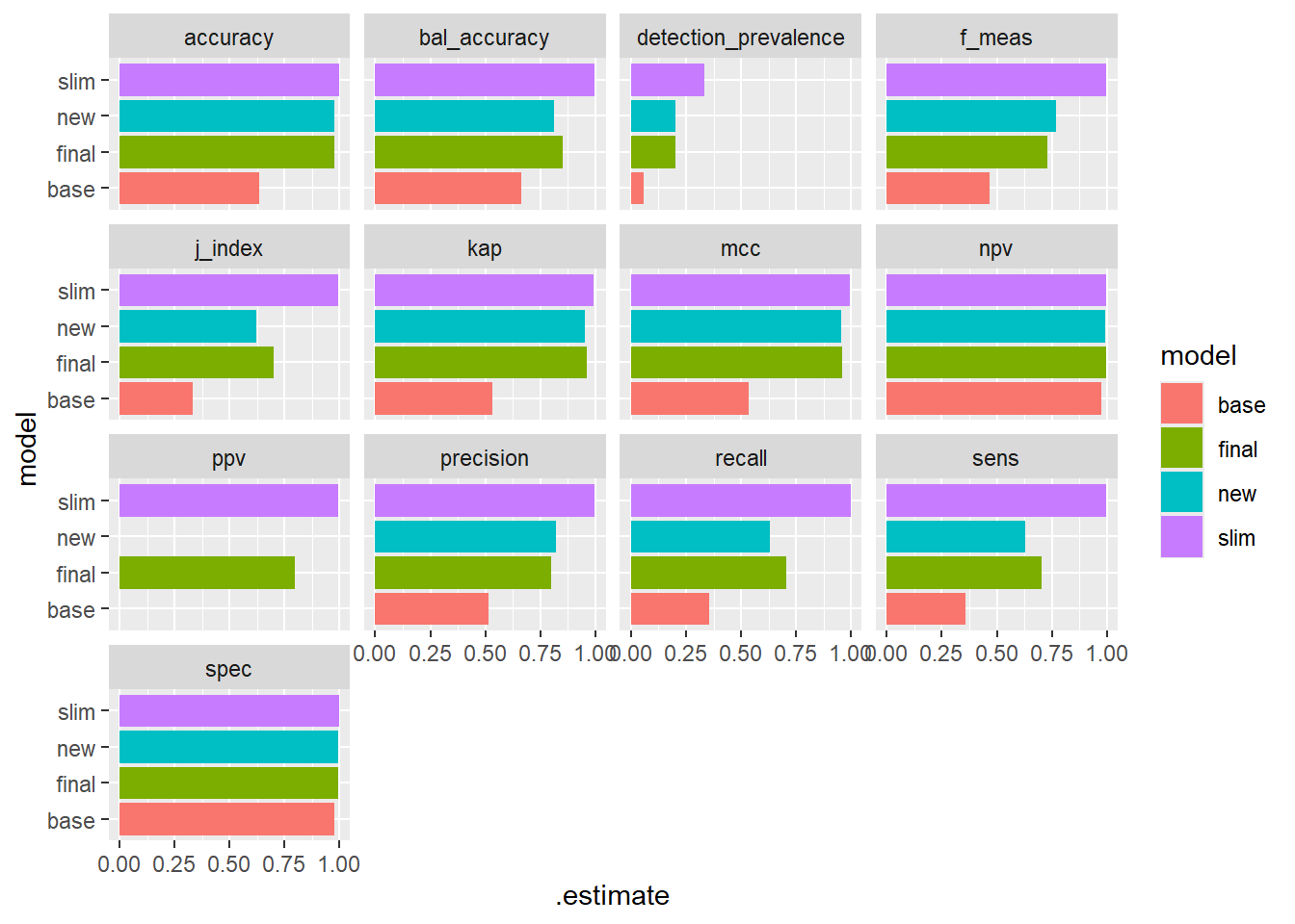
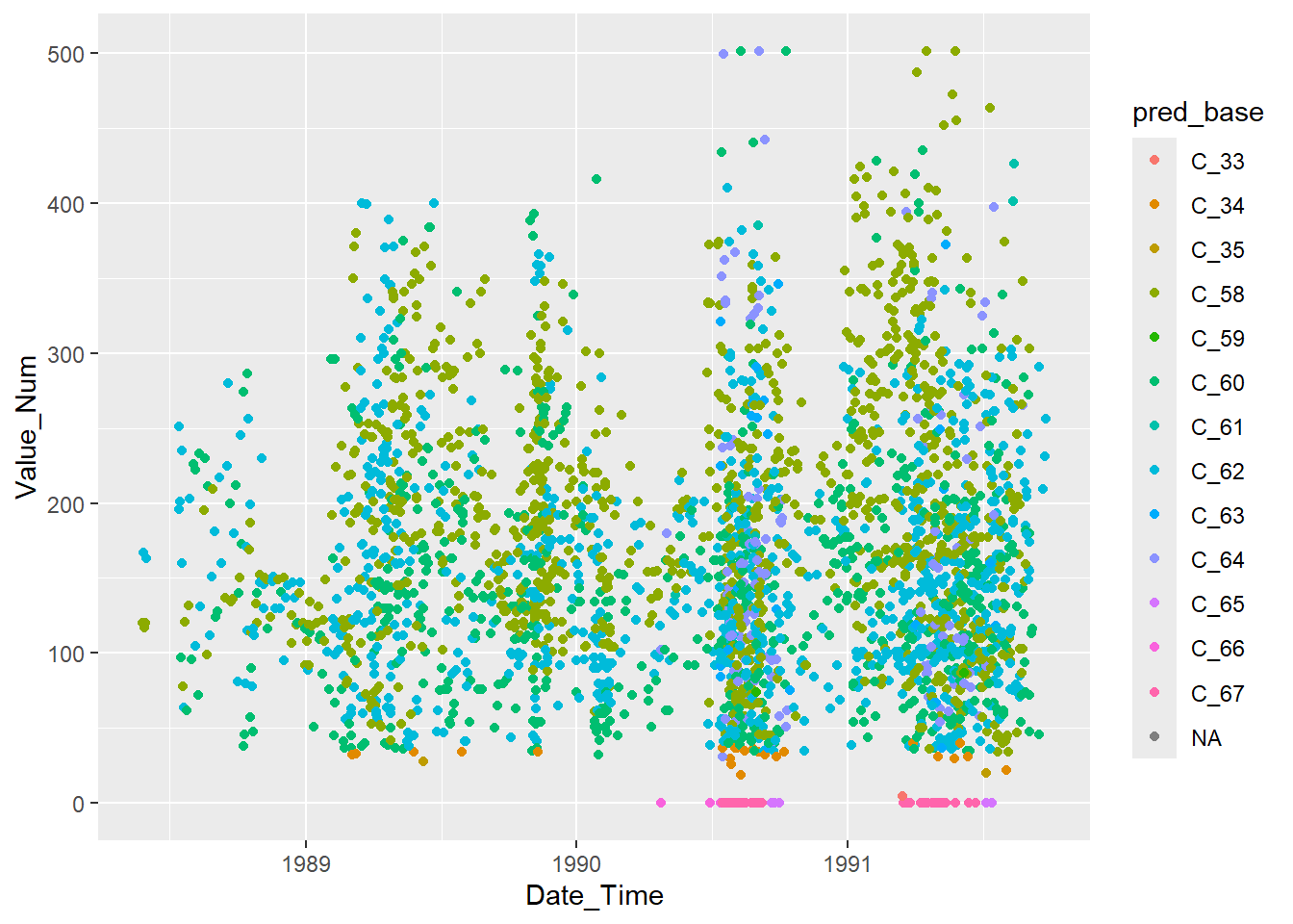
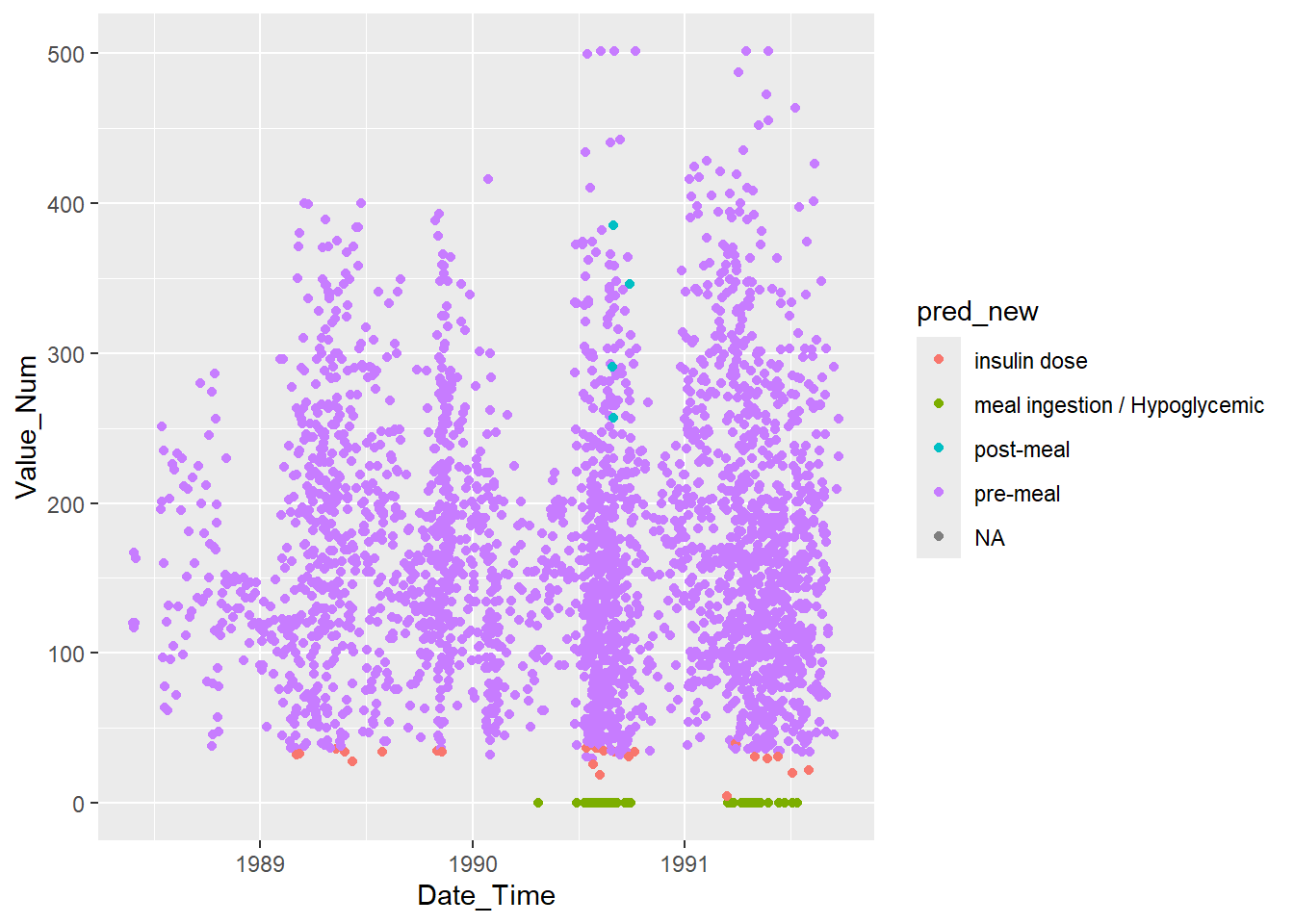
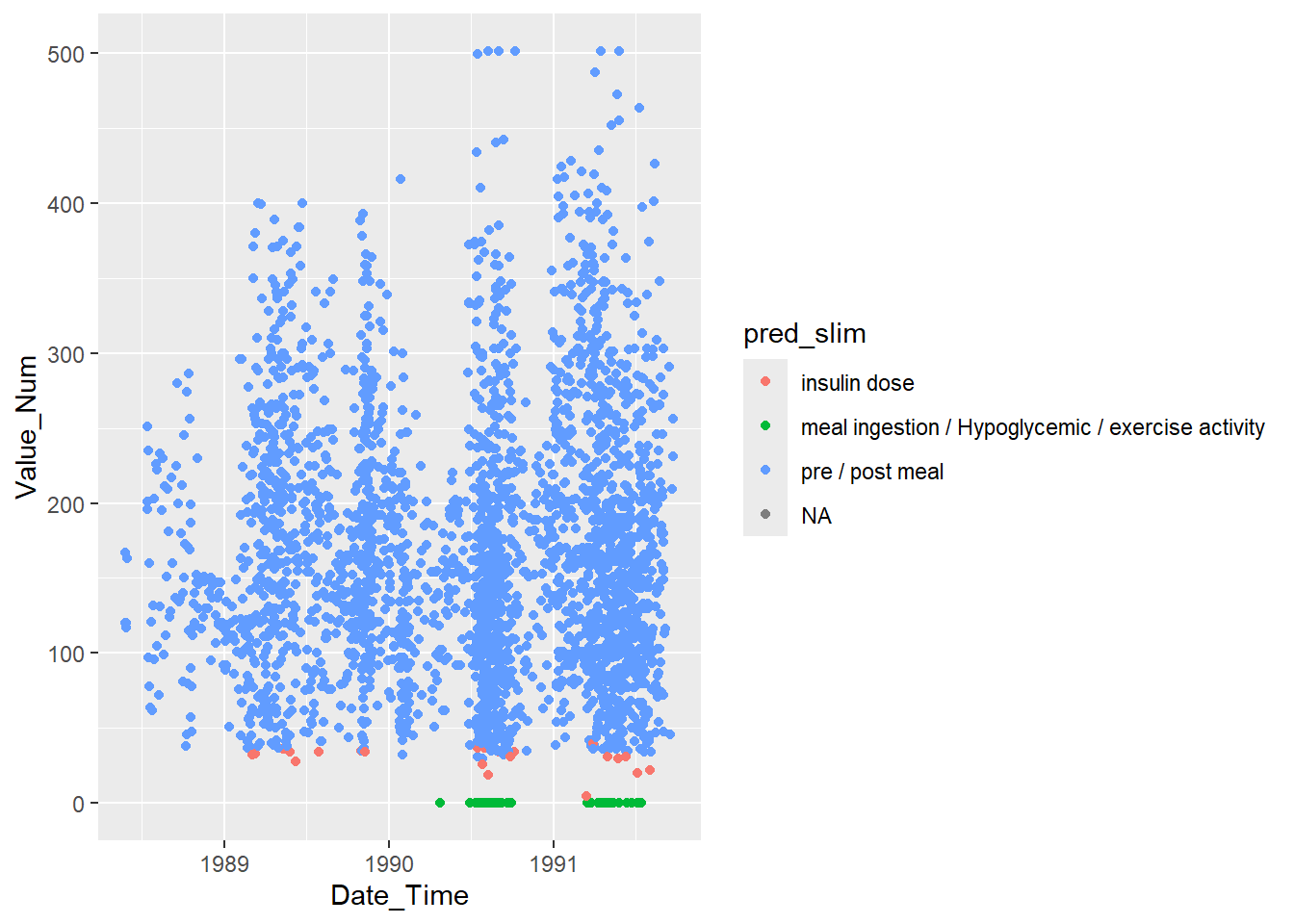
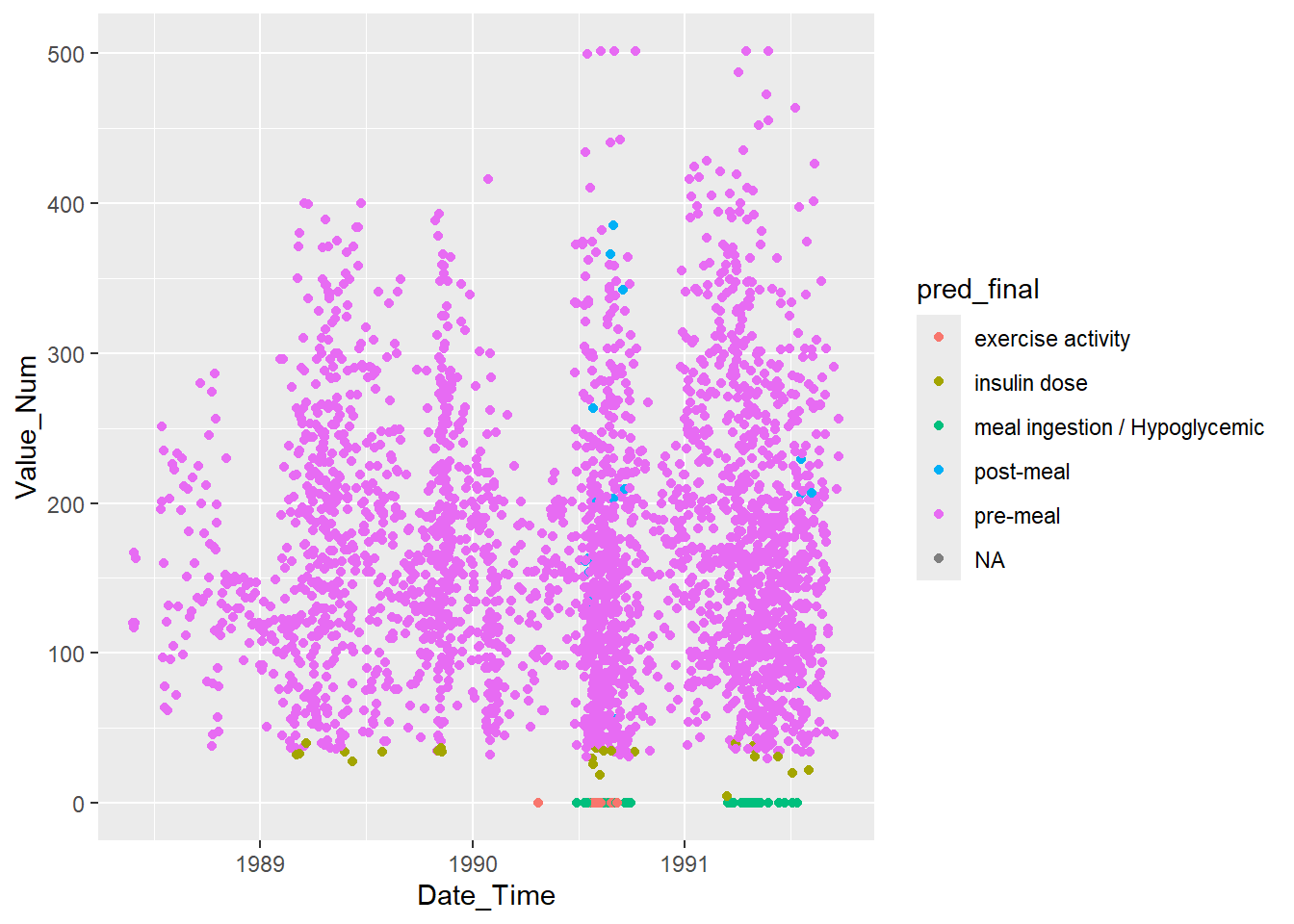
Project UnKnown Data with Final Model
Source Code
# Random Forest Date/Time Modeling Example {#sec-diabetic-monitoring}Diabetes date/time-stamped data shall be analyzed using the random forest method. The DIABETES data sets are provided for use in 1994 AI in Medicine symposium submissions (AIM-94 data set provided by Michael Kahn, MD, PhD, Washington University, St. Louis, MO) and may be downloaded from [https://archive.ics.uci.edu/ml/datasets/Diabetes](https://archive.ics.uci.edu/ml/datasets/Diabetes). The DIABETES data contain:- Data-Codes: a listing of the codes used in the data sets.- Domain-Description: This file describes the basic physiology and patho-physiology of diabetes mellitus and its treatment.- data-\[01-70\]: data sets covering several weeks' to months' worth of outpatient care on 70 patients.The folder `Diabetes-Data` is referenced from [https://archive.ics.uci.edu/ml/datasets/Diabetes](https://archive.ics.uci.edu/ml/datasets/Diabetes) as per the website> ## **Diabetes Data Set**> Diabetes Data Set Download: [Data Folder](https://archive.ics.uci.edu/ml/machine-learning-databases/diabetes/), Data Set Description>> **Abstract**: This diabetes dataset is from AIM '94>> +--------------------------------+---------------------------+---------------------------+----------+-------------------------+------------------------------+> | **Data Set Characteristics:** | Multivariate, Time-Series | **Number of Instances:** | ? | **Area:** | Life |> +--------------------------------+---------------------------+---------------------------+----------+-------------------------+------------------------------+> | **Attribute Characteristics:** | Categorical, Integer | **Number of Attributes:** | 20 | **Date Donated** | Not Reported |> +--------------------------------+---------------------------+---------------------------+----------+-------------------------+------------------------------+> | **Associated Tasks:** | | **Missing Values?** | ? | **Number of Web Hits:** | 561559 |> | | | | | | |> | | | | | | as reported on of April 2021 |> +--------------------------------+---------------------------+---------------------------+----------+-------------------------+------------------------------+>> : Characteristics of Diabetes Data Set on <https://archive.ics.uci.edu/ml/datasets/Diabetes>>> **Source:** Michael Kahn, MD, PhD, Washington University, St. Louis, MO> **Data Set Information:** Diabetes patient records were obtained from two sources: an automatic electronic recording device and paper records. The automatic device had an internal clock to timestamp events, whereas the paper records only provided "logical time" slots (breakfast, lunch, dinner, bedtime). For paper records, fixed times were assigned to breakfast (08:00), lunch (12:00), dinner (18:00), and bedtime (22:00). Thus paper records have fictitious uniform recording times whereas electronic records have more realistic time stamps.>> Diabetes files consist of four fields per record. Each field is separated by a tab and each record is separated by a newline.>> File format:>> 1. Date in MM-DD-YYYY format> 2. Time in XX:YY format> 3. Code> 4. Value>> The Code field is deciphered as follows:>> - 33 = Regular insulin dose> - 34 = NPH insulin dose> - 35 = UltraLente insulin dose> - 48 = Unspecified blood glucose measurement> - 57 = Unspecified blood glucose measurement> - 58 = Pre-breakfast blood glucose measurement> - 59 = Post-breakfast blood glucose measurement> - 60 = Pre-lunch blood glucose measurement> - 61 = Post-lunch blood glucose measurement> - 62 = Pre-supper blood glucose measurement> - 63 = Post-supper blood glucose measurement> - 64 = Pre-snack blood glucose measurement> - 65 = Hypoglycemic symptoms> - 66 = Typical meal ingestion> - 67 = More-than-usual meal ingestion> - 68 = Less-than-usual meal ingestion> - 69 = Typical exercise activity> - 70 = More-than-usual exercise activity> - 71 = Less-than-usual exercise activity> - 72 = Unspecified special event# Download DataOur first task is to use R to download the data.The code below creates a temporary directory within the current project directory, downloads a compressed file from a URL to that temporary directory, and then extracts the contents of the compressed file into the same temporary directory.```{r}#| label: download-data-ucitemp_path <-"Temp_DM_Path"#This line creates a new directory with the path specified by file.path(here::here(),temp_path). The here::here() function returns the path to the current project directory, and file.path combines this with the value of temp_path to create the full path to the new temporary directory.dir.create(file.path(here::here(),temp_path)) my_tar_file <-file.path(here::here(),temp_path,'diabetes-data.tar.Z')# This line creates a variable my_url and assigns it the value of a URL that points to a compressed file.my_url <-'https://archive.ics.uci.edu/ml/machine-learning-databases/diabetes/diabetes-data.tar.Z'# This line downloads the file from the URL specified by my_url and saves it to the local path specified by my_tar_file. The mode = "wb" argument specifies that the file should be saved in binary mode.download.file(my_url, my_tar_file,mode ="wb") # This line uses the archive_extract function from the archive package to extract the contents of the compressed file specified by my_tar_file into the directory specified by dir= file.path(here::here(),temp_path), which is the same temporary directory created in step 2.archive::archive_extract(my_tar_file, dir=file.path(here::here(),temp_path)) ```## Load DataOur analysis begins with file path definitions followed by the `read_in_text_from_file_no` function used to import the diabetes data.```{r}#| label: DM2-TS-pathDM2_TS_path <- here::here("Temp_DM_Path/Diabetes-Data")```We then create a list of file paths ```{r list_of_file_paths}list_of_file_paths <- list.files(path = DM2_TS_path, pattern = 'data-', recursive = TRUE, full.names = TRUE)head(list_of_file_paths)length(list_of_file_paths)``````{r}library('stringr')library('tidyverse')tibble_of_file_paths <-tibble(list_of_file_paths) %>%mutate(full_path = list_of_file_paths) %>%mutate(file_no =str_replace(string = full_path,pattern =paste0(here::here("Temp_DM_Path/Diabetes-Data"),'/data-'),replacement ='')) tibble_of_file_paths |>head()``````{r 5-read-data-function }read_in_text_from_file_no <- function(my_file_no){ enquo_by <- enquo(my_file_no) cur_file <- tibble_of_file_paths %>% filter(file_no == !!enquo_by) cur_path <- as.character(cur_file$full_path) dat <- readr::read_tsv(cur_path, col_names = c('Date',"Time","Code","Value"), col_types = cols(col_character(), col_character(), col_character(), col_character()) ) %>% mutate(file_no = as.numeric(cur_file$file_no)) return(dat)}```The goal of using purrr functions instead of for loops is to allow you to break common list manipulation challenges into independent pieces:How can you solve the problem for a single element of the list? Once you’ve solved that problem, purrr takes care of generalizing your solution to every element in the list.If you’re solving a complex problem, how can you break it down into bite-sized pieces that allow you to advance one small step towards a solution? With purrr, you get lots of small pieces that you can compose together with the pipe.This structure makes it easier to solve new problems. It also makes it easier to understand your solutions to old problems when you re-read your old code.purrr functions are implemented in C making them very fast.```{r 5-furrr-2 }DM2_TIME_RAW <- purrr::map_dfr(tibble_of_file_paths$file_no, # list of columns function(x){ read_in_text_from_file_no(x) })```Since we have saved the data as an RDS we can remove the temporary files:```{r}unlink(here::here(temp_path), recursive =TRUE)```The data are a matrix (data.frame) of 29,330 rows and 5 columns. The column names are `Date` (character of mm-dd-yyy), `Time` (character of h:mm and hh:mm), `Code` (character of two-digit numbers), `Value` (character of three-digit numbers), and `file_no` (number from `r min(DM2_TIME_RAW$file_no)` to `r max(DM2_TIME_RAW$file_no)`). The Code number definitions are listed in the R script listing below and are referenced by the `Code_Table` tibble we define below. ```{r 5-code-table }Code_Table <- tribble( ~ Code, ~ Code_Description, 33 , "Regular insulin dose", 34 , "NPH insulin dose", 35 , "UltraLente insulin dose", 48 , "Unspecified blood glucose measurement", # This decode value is the same as 57 57 , "Unspecified blood glucose measurement", # This decode value is the same as 48 58 , "Pre-breakfast blood glucose measurement", 59 , "Post-breakfast blood glucose measurement", 60 , "Pre-lunch blood glucose measurement", 61 , "Post-lunch blood glucose measurement", 62 , "Pre-supper blood glucose measurement", 63 , "Post-supper blood glucose measurement", 64 , "Pre-snack blood glucose measurement", 65 , "Hypoglycemic symptoms", 66 , "Typical meal ingestion", 67 , "More-than-usual meal ingestion", 68 , "Less-than-usual meal ingestion", 69 , "Typical exercise activity", 70 , "More-than-usual exercise activity", 71 , "Less-than-usual exercise activity", 72 , "Unspecified special event") %>% # What does this mean? mutate(Code_Invalid = if_else(Code %in% c(48,57,72), TRUE, FALSE)) %>% mutate(Code_New = if_else(Code_Invalid == TRUE, 999, Code)) Code_Table```Data conditioning, i.e., defining and redefining the data types by column is given in the listing below.The codes in `Code_Table` are converted into factor data with code number 72, "Unspecified special event", removed.```{r 5-code-table-factor }Code_Table_Factor <- Code_Table %>% filter(Code_Invalid == FALSE) %>% mutate(Code_Factor = factor(paste0("C_",Code_New)))Code_Table_Factor``````{r 5-lubridate }library('lubridate')DM2_TIME <- DM2_TIME_RAW %>% mutate(Date_Time_Char = paste0(Date, ' ', Time)) %>% mutate(Date_Time = mdy_hm(Date_Time_Char)) %>% mutate(Value_Num = as.numeric(Value)) %>% mutate(Code = as.numeric(Code)) %>% mutate(Record_ID = row_number()) %>% left_join(Code_Table_Factor)DM2_TIME```The result is the raw, imported data in `DM2_TIME_RAW` are conditioned, assigned to object `DM2_TIME`, and `DM2_TIME_RAW` is removed from the computing environment. The conditioning combines the dates in the Date column with the times in the Time are combined into a date time string, `Date_Time_Char` (mm-dd-yyyy h:mm or hh:mm), which then is converted into the date time format yyyy-mm-dd hh:mm:ss in column `Date_Time`. The numeric value of the character Value is assigned to column `Value_Num`. The character form of the codes in Code are redefined as numeric. A new column, `Record_ID`, is assigned the row number (1 to 29,330).To ascertain if the complete records are indeed complete, a bar plot showing the percent complete for value number (blue), date and time (green), and code (red) is shown in Figure \ref{fig:Per_Complete}. The abscissa is the percent complete from 0 to 100. ```{r 5-features-pct-complete-fun }Features_Percent_Complete <- function(data, Percent_Complete = 0){ SumNa <- function(col){sum(is.na(col))} na_sums <- data %>% summarise_all(SumNa) %>% tidyr::pivot_longer(everything() ,names_to = 'feature', values_to = 'SumNa') %>% arrange(-SumNa) %>% mutate(PctNa = SumNa/nrow(data)) %>% mutate(PctComp = (1 - PctNa)*100) data_out <- na_sums %>% filter(PctComp >= Percent_Complete)return(data_out)}``````{r 5-percent-complete-graph }Feature_Percent_Complete_Graph <- function(data, Percent_Complete = 0 ){ table <- Features_Percent_Complete(data, Percent_Complete) plot1 <- table %>% mutate(feature = reorder(feature, PctComp)) %>% ggplot(aes(x=feature, y =PctComp, fill=feature)) + geom_bar(stat = "identity") + coord_flip() + theme(legend.position = "none") return(plot1)} ``````{r 5-percent-complete-graph-1 , fig.cap="DM2 TIME Feature % Complete Graph"}Feature_Percent_Complete_Graph(data = DM2_TIME %>% select(Date_Time, Value_Num, Code_Factor) )```Examination of the data reveal not all records are complete. The section of code identifies these records after joining the data with the scrubbed code table data. The unknown measurement data are assigned to the `Unknown_Measurements` object.```{r 5-def-unk }UnKnown_Measurements <- DM2_TIME %>% filter(is.na(Code_Factor) | is.na(Date_Time) | is.na(Value_Num) | Code_Invalid == TRUE | Code_New == 999 )UnKnown_Measurements```Similarly, complete records are assigned to the `Known_Measurements` object. The data in this object are plotted (Figure \ref{fig:known_measures}) with `Value_Num` on the ordinate and `Date_Time` (year) on the abscissa. The legend is color coded by `Code`. ```{r 5-def-known }Known_Measurements <- DM2_TIME %>% anti_join(UnKnown_Measurements %>% select(Record_ID)) Known_Measurements```We see the three variables are 100\% complete within the Known_Measurements:```{r 5-percent-complete-graph-2 , fig.cap="Known Measurements Feature % Complete Graph"}Feature_Percent_Complete_Graph(data = Known_Measurements %>% select(Date_Time, Value_Num, Code_Factor) )```## View Data```{r 5-view-known }Known_Measurements %>% ggplot(aes(x=Date_Time, y=Value_Num, color=Code_Factor)) + geom_point()```## UnKnown MeasurementsWe can take a look at the UnKnown Measurements below, R will give us a warning that there are `r UnKnown_Measurements %>% filter(is.na(Date_Time) | is.na(Value_Num)) %>% tally() %>% pull(n)` which either have missing `Date_Time` or missing `Value_Num`.```{r 5-unknown-fig-1 , fig.cap="UnKnown Measurements"}UnKnown_Measurements %>% ggplot(aes(x=Date_Time, y=Value_Num)) + geom_point() ```We will make it our prediction task to classify the UnKnown_Measurements. ## Split Training Data```{r 5-train-test-split }set.seed(123)train_records <- sample(Known_Measurements$Record_ID, size = nrow(Known_Measurements)*.6, replace = FALSE)train <- Known_Measurements %>% filter(Record_ID %in% train_records)test <- Known_Measurements %>% filter(!(Record_ID %in% train_records))``````{r 5-train-graph, fig.cap="Plot of Training Data"}train %>% ggplot(aes(x=Date_Time, y=Value_Num, color=Code_Factor)) + geom_point() ``````{r 5-test-data-graph, fig.cap="Plot of Test Data"}test %>% ggplot(aes(x=Date_Time, y=Value_Num, color=Code_Factor)) + geom_point() ```## Fit Model 1```{r 5-rf-1}library('randomForest')rf_model <- randomForest(Code_Factor ~ Date_Time + Value_Num, data = train, ntree = 659, importance = TRUE)```### Random Forest OuputHere's the output of Random Forest```{r 5-rf-1-out }rf_model```The Confusion Matrix that we see above is the confusion matrix from fitting the model against the training data so it is overly optimistic in terms of predictions.Random Forest is a collection of Decision Trees, we can look at the individual trees in the forest by using one of the two following functions.```{r 5-ggraph }library(ggraph)library(igraph)``````{r 5-plot-rf-tree }plot_rf_tree <- function(final_model, tree_num, shorten_label = TRUE) { # get tree by index tree <- randomForest::getTree(final_model, k = tree_num, labelVar = TRUE) %>% tibble::rownames_to_column() %>% # make leaf split points to NA, so the 0s won't get plotted mutate(`split point` = ifelse(is.na(prediction), `split point`, NA)) # prepare data frame for graph graph_frame <- data.frame(from = rep(tree$rowname, 2), to = c(tree$`left daughter`, tree$`right daughter`)) # convert to graph and delete the last node that we don't want to plot graph <- graph_from_data_frame(graph_frame) %>% delete_vertices("0") # set node labels V(graph)$node_label <- gsub("_", " ", as.character(tree$`split var`)) if (shorten_label) { V(graph)$leaf_label <- substr(as.character(tree$prediction), 1, 1) } V(graph)$split <- as.character(round(tree$`split point`, digits = 2)) # plot plot <- ggraph(graph, 'tree') + theme_graph() + geom_edge_link() + geom_node_point() + geom_node_label(aes(label = leaf_label, fill = leaf_label), na.rm = TRUE, repel = FALSE, colour = "white", show.legend = FALSE) print(plot)}``````{r 5-tree-456-2}plot_rf_tree(rf_model, 456)```Random Forest models normally come equipped with feature importances which we can access with the `varImpPlot` function in this instance:```{r 5-varImpPlot, fig.cap="Feature Importances of Base Model"}varImpPlot(rf_model)```For instance, above we see that `Date_Time` is more important in terms classifying the measurement as opposed to `Value_Num`We can also extract the feature importances for each of the classes:```{r 5-varImp-caret }caret::varImp(rf_model, scale = FALSE) %>% t() %>% # transpose the entire dataframe as_tibble(rownames = 'Class' ) # turn it back to a tibble```The Random Forest model also has a plot associated with it:```{r 5-plot-rf, fig.cap= "plot of randomForest model output"}plot(rf_model)```Let's see if we can figure out what is going on with the above graph. We can extract the `err.rate` and `ntree` from the model object and place them in a `matplot` to match the above graph.```{r 5-derivation, fig.cap="derivation of plot of randomForest model output"}err <- rf_model$err.rateN_trees <- 1:rf_model$ntreematplot(N_trees , err, type = 'l', xlab="trees", ylab="Error")```We can improve this a bit by performing the computations ourselves and keeping track of things:```{r 5-err-levels }err2 <- as_tibble(err, rownames='n_trees')err2 %>% glimpse()predicted_levels <- colnames(err2)[!colnames(err2) %in% c('n_trees','OOB')]predicted_levels``````{r 5-plot-rf1-err-ggplot, fig.cap="Improved plot of base randomForest model output"}plot <- err2 %>% select(-OOB) %>% pivot_longer(all_of(predicted_levels), names_to = "Class", values_to = "Error") %>% mutate(N_Trees = as.numeric(n_trees)) %>% ggplot(aes(x=N_Trees, y=Error, color=Class)) + geom_point() + geom_smooth(method = lm, formula = y ~ splines::bs(x, 3), se = FALSE) plot``````{r better-rf-plot }better_rand_forest_errors <- function(rf_model_obj){ err <- rf_model_obj$err.rate err2 <- as_tibble(err, rownames='n_trees') predicted_levels <- colnames(err2)[!colnames(err2) %in% c('n_trees','OOB')] plot <- err2 %>% select(-OOB) %>% pivot_longer(all_of(predicted_levels), names_to = "Class", values_to = "Error") %>% mutate(N_Trees = as.numeric(n_trees)) %>% ggplot(aes(x=N_Trees, y=Error, color=Class)) + geom_point() + geom_smooth(method = lm, formula = y ~ splines::bs(x, 3), se = FALSE) return(plot)}```## Evaluate Model Performace```{r 5-score-test-base-1}test_Scored <- test %>% mutate(model = 'base')```First, we will get the expected classes for the test data:```{r 5-score-test-base-2}test_Scored$pred <- predict(rf_model, test , 'response')test_Scored %>% glimpse()``````{r 5-score-test-base-3}library('yardstick')test_Scored %>% conf_mat(truth = Code_Factor, pred) %>% autoplot('mosaic')``````{r 5-mm-1 , fig.cap="Model Evaluation Metrics - Base Model"}test_Scored %>% conf_mat(truth= Code_Factor, pred) %>% summary() %>% ggplot(aes(x=.metric, y=.estimate, fill= .metric)) + geom_bar(stat='identity', position = 'dodge') + coord_flip()``````{r 5-predict-true-falue-rf-1, fig.cap="Graph of Correct Predictions on test data under base model" }test_Scored %>% mutate(Predict_Correct = if_else(Code_Factor == pred, TRUE, FALSE)) %>% ggplot(aes(x=Date_Time, y=Value_Num, color=Predict_Correct)) + geom_point() ```## Correlated ProbabilitesFirst, let's review the probabilities:```{r 5-rf1-probs }Probs <- predict(rf_model, test_Scored, 'prob') %>% as_tibble() Probstest_Scored <- cbind(test_Scored, Probs)``````{r 5-ggalyy-probs }GGally::ggcorr(Probs, method = c("pairwise", "pearson"), label = TRUE)``````{r 5-corrr-data }library('corrr')corr_data <- correlate(Probs, use = "pairwise.complete.obs", method = "pearson",)corr_data %>% glimpse()``````{r 5-corrr-data-heatmap , fig.cap="Heatmap Confusion Matrix of base model"}test_Scored %>% conf_mat(truth = Code_Factor, pred) %>% autoplot('heatmap')```One of the things to note above is that classes `C_68`, `C_69`, `C_70`, `C_71` are never predicted.Likewise the probabilities of `C_65`, `C_70`, and `C_67` are highly correlated:```{r 5-corr-all-probs }corr_data %>% filter_at(vars(all_of(colnames(Probs))), any_vars( . > .6 ))```And there are a number of classes which do not have many training examples:```{r 5-small-training-classes }train %>% group_by(Code_Factor) %>% tally() %>% ungroup() %>% mutate(n = as.numeric(n)) %>% full_join(Code_Table_Factor) %>% mutate(n = if_else(is.na(n) , 0 , n)) %>% arrange(n) %>% print(n=20)```To aide us further, we will perform a k-means clustering on the probabilities to get a sense of how many classes we should have. Our first step in this endeavor will be to create a sample of roughly `60 %` of the available probabilities:```{r 5-sample-probs}Probs_sample <- Probs %>% rowwise() %>% mutate(rand_num = runif(1)) %>% ungroup() %>% filter(rand_num > .4) %>% select(-rand_num) # this should sample roughly 60% of the Probs data nrow(Probs_sample)/nrow(Probs) ``````{r 5-proc-kmeans , cache=FALSE}library('broom')proc.kmeans <- function(data, k = 1:9){kclusts <- tibble(k = k) %>% mutate( kclust = map(k, ~kmeans(data, .x)), glanced = map(kclust, glance), augmented = map(kclust, augment, data) )kmeans_model <- function(final_k = 5){ (kclusts %>% filter(k == final_k))$kclust[[1]]}id_vars <- colnames(kclusts)cluster_assignments <- kclusts %>% unnest(cols = augmented)vars <- setdiff(colnames(cluster_assignments), c(id_vars,'.cluster'))within_cluster_variation_plot <- kclusts %>% unnest(cols = c(glanced)) %>% ggplot(aes(k, tot.withinss)) + geom_line() + geom_point() + scale_x_continuous(breaks = scales::pretty_breaks(n = max(k))) + labs(title = "Within Cluster Variation versus number of Clusters")kmeans.pca <- cluster_assignments %>% select(all_of(vars)) %>% prcomp()cluster_assignments_plot <- kmeans.pca %>% augment(cluster_assignments) %>% ggplot( aes(x = .fittedPC1, y = .fittedPC2, color = .cluster )) + geom_point(alpha = 0.8) + facet_wrap(~ k) + labs(title = "k-means clusterings")return(list(cluster_assignments_plot= cluster_assignments_plot, within_cluster_variation_plot=within_cluster_variation_plot, kmeans_model = kmeans_model))}``````{r 5-fviz_nbclust-probs , cache=FALSE}proc.kmeans.results <- proc.kmeans(Probs_sample, k=3:11)proc.kmeans.results``````{r}proc.kmeans.results$kmeans_model(6) %>%augment(Probs_sample) %>%rownames_to_column("id") %>%pivot_longer(cols =c(-.cluster, -id), names_to ="class", values_to ="prob") %>%mutate(prob =as.numeric(prob)) %>%arrange(desc(prob)) %>%ggplot(aes(x=class, y=prob, color = .cluster)) +geom_point() +facet_wrap(~.cluster)``````{r}proc.kmeans.results$kmeans_model(6) %>%augment(Probs_sample) %>%rownames_to_column("id") %>%pivot_longer(cols =c(-.cluster, -id), names_to ="class", values_to ="prob") %>%mutate(prob =as.numeric(prob)) %>%arrange(desc(prob)) %>%filter(.cluster ==5) %>%ggplot(aes(x=class, y=prob, color = .cluster)) +geom_point() ``````{r}rm(proc.kmeans.results)saveRDS(rf_model, here::here("DATA/Part_5/models/rf_model.RDS"))rm(rf_model)```## Make AdjustmentsOur previous model has some issues, which we can attempt to correct.```{r 5-cf2 }Code_Table_Factor_2 <- Code_Table_Factor %>% mutate(Code_Description_2 = case_when( Code %in% c(33, 34, 35) ~ "insulin dose", Code %in% c(58, 60, 62, 64) ~ "pre-meal", Code %in% c(59, 61, 63) ~ "post-meal", Code %in% c(66, 67, 68, 65) ~ "meal ingestion / Hypoglycemic", Code %in% c(69, 70, 71) ~ "exercise activity") ) %>% mutate(Code_Description_2 = factor(Code_Description_2)) %>% select(Code, Code_Description_2)Code_Table_Factor_2``````{r 5-rf2-train }train_2 <- train %>% left_join(Code_Table_Factor_2)rf_model_2 <- randomForest(Code_Description_2 ~ Date_Time + Value_Num, data = train_2, ntree = 659, importance = TRUE)``````{r 5-better-rand-errors-rf-2 , fig.cap="Training Errors on New Model"}better_rand_forest_errors(rf_model_2)``````{r 5-heatmap-conf-mat-rf-2 , fig.cap="Heatmap Confusion Matrix of New Model"}test_Scored2 <- test %>% left_join(Code_Table_Factor_2) %>% mutate(model = 'new')test_Scored2$pred <- predict(rf_model_2, test_Scored2 , 'response')conf_mat.test_Scored2 <- test_Scored2 %>% conf_mat(truth = Code_Description_2, pred)conf_mat.test_Scored2 %>% autoplot('heatmap')``````{r}saveRDS(rf_model_2, here::here('DATA/Part_5/models/rf_model_2.RDS'))``````{r 5-compare-rf12 ,fig.cap="Model Evaluation Metrics - base Vs new model"}base <- test_Scored %>% conf_mat(truth= Code_Factor, pred) %>% summary() %>% mutate(model = 'base')new <- test_Scored2 %>% conf_mat(truth= Code_Description_2, pred) %>% summary() %>% mutate(model = 'new')comp <- bind_rows(base, new)comp %>% ggplot(aes(x=model, y=.estimate, fill= model)) + geom_bar(stat='identity', position = 'dodge') + coord_flip() + facet_wrap(.metric ~ .)```## Make Adjustments, AgainLet's make another pass at this, this time we will group together```{r 5-code_table-3 }Code_Table_Factor_3 <- Code_Table_Factor %>% mutate(Code_Description_3 = case_when( Code %in% c(33, 34, 35) ~ "insulin dose", Code %in% c(58, 60, 62, 64, 59, 61, 63) ~ "pre / post meal", Code %in% c(66, 67, 68, 65, 69, 70, 71) ~ "meal ingestion / Hypoglycemic / exercise activity")) %>% mutate(Code_Description_3 = factor(Code_Description_3)) %>% select(Code, Code_Description_3)Code_Table_Factor_3``````{r 5-rf-3-train }train_3 <- train %>% left_join(Code_Table_Factor_3)rf_model_3 <- randomForest(Code_Description_3 ~ Date_Time + Value_Num, data = train_3, ntree = 659, importance = TRUE)``````{r}rm(train_3)``````{r 5-rf-train-errors, fig.cap="Training Errors of Final Model"}better_rand_forest_errors(rf_model_3)``````{r 5-heatmap-cf-model-rf3 , fig.cap="Heatmap Confusion Matrix of Final Model"}test_Scored3 <- test %>% left_join(Code_Table_Factor_3) %>% mutate(model = 'final')test_Scored3$pred <- predict(rf_model_3, test_Scored3 , 'response')conf_mat.test_Scored3 <- test_Scored3 %>% conf_mat(truth = Code_Description_3, pred)conf_mat.test_Scored3 %>% autoplot('heatmap')``````{r}saveRDS(rf_model_3, here::here('DATA/Part_5/models/rf_model_3.RDS'))rm(rf_model_3)```## Extract More Data```{r}library('ggplot2')library('ggdendro')library('tree')tree_1 <- tree::tree(Code_Factor ~ Date_Time + Value_Num, data = train)plot_dendro_tree <-function(model){ tree_data <-dendro_data(model)p <-segment(tree_data) %>%ggplot() +geom_segment(aes(x = x, y = y, xend = xend, yend = yend, size = n), colour ="blue", alpha =0.5) +scale_size("n") +geom_text(data =label(tree_data), aes(x = x, y = y, label = label), vjust =-0.5, size =3) +geom_text(data =leaf_label(tree_data), aes(x = x, y = y, label = label), vjust =0.5, size =2) +theme_dendro()p}plot_dendro_tree(tree_1)tree_2 <- tree::tree(Code_Factor ~ Date_Time + Value_Num + h + day + month , data = train_2 %>%mutate(h =factor(lubridate::hour(Date_Time))) %>%select(Code_Factor, Date_Time, Value_Num, h) %>%mutate(day = lubridate::day(Date_Time)) %>%mutate(month =month(Date_Time, label =TRUE)) )plot_dendro_tree(tree_2)``````{r}rf_model_4 <-randomForest(Code_Description_2 ~ Date_Time + Value_Num + h + day + month,data = train_2 %>%mutate(h =factor(lubridate::hour(Date_Time))) %>%select(Code_Description_2, Code_Factor, Date_Time, Value_Num, h) %>%mutate(day = lubridate::day(Date_Time)) %>%mutate(month =month(Date_Time, label =TRUE)),ntree =659,importance =TRUE)``````{r}better_rand_forest_errors(rf_model_4)``````{r}test_Scored4 <- test %>%left_join(Code_Table_Factor_2) %>%mutate(model ='final') %>%mutate(h =factor(lubridate::hour(Date_Time))) %>%mutate(day = lubridate::day(Date_Time)) %>%mutate(month =month(Date_Time, label =TRUE)) %>%select(Code_Description_2, Code_Factor, Date_Time, Value_Num, day, month, h) test_Scored4$pred <-predict(rf_model_4, test_Scored4 , 'response')conf_mat.test_Scored4 <- test_Scored4 %>%conf_mat(truth = Code_Description_2, pred)``````{r 5-compare-base-new-final, fig.cap="Model Evaluation Metrics - base Vs new model Vs Final"}slim <- conf_mat.test_Scored3 %>% summary() %>% mutate(model = 'slim')final <- conf_mat.test_Scored4 %>% summary() %>% mutate(model = 'final')comp_f <- bind_rows(comp, slim, final)comp_f %>% ggplot(aes(x=model, y=.estimate, fill = model)) + geom_bar(stat='identity', position = 'dodge') + coord_flip() + facet_wrap(.metric ~ .)```## Predict UnKnown Data```{r}keep =c('UnKnown_Measurements','rf_model','rf_model_2','rf_model_3','rf_model_4','keep')rm(list =setdiff(ls(), keep))rf_model <-readRDS(here::here('DATA/Part_5/models/rf_model.RDS'))rf_model_2 <-readRDS(here::here('DATA/Part_5/models/rf_model_2.RDS'))rf_model_3 <-readRDS(here::here('DATA/Part_5/models/rf_model_3.RDS'))``````{r}UnKnown_Measurements$pred_base <-predict(rf_model, UnKnown_Measurements , 'response')UnKnown_Measurements$pred_new <-predict(rf_model_2, UnKnown_Measurements , 'response')UnKnown_Measurements$pred_slim <-predict(rf_model_3, UnKnown_Measurements , 'response')UnKnown_Measurements <- UnKnown_Measurements %>%mutate(h =factor(lubridate::hour(Date_Time))) %>%mutate(day = lubridate::day(Date_Time)) %>%mutate(month =month(Date_Time, label =TRUE))UnKnown_Measurements$pred_final <-predict(rf_model_4, UnKnown_Measurements, 'response')``````{r 5-unknown-base, fig.cap="Project UnKnown Data with Base Model"}UnKnown_Measurements %>% ggplot(aes(x=Date_Time, y=Value_Num, color=pred_base)) + geom_point()``````{r 5-unknown-new, fig.cap="Project UnKnown Data with New Model"}UnKnown_Measurements %>% ggplot(aes(x=Date_Time, y=Value_Num, color=pred_new)) + geom_point()``````{r 5-unknown-slim, fig.cap="Project UnKnown Data with slim Model"}UnKnown_Measurements %>% ggplot(aes(x=Date_Time, y=Value_Num, color=pred_slim)) + geom_point()``````{r 5-unknown-final, fig.cap="Project UnKnown Data with Final Model"}UnKnown_Measurements %>% ggplot(aes(x=Date_Time, y=Value_Num, color=pred_final)) + geom_point()```