Joining with `by = join_by(SEQN)`
Joining with `by = join_by(SEQN)`
Joining with `by = join_by(SEQN)`
Joining with `by = join_by(SEQN)`
Joining with `by = join_by(SEQN)`
Joining with `by = join_by(SEQN)`
Joining with `by = join_by(SEQN)`
Joining with `by = join_by(SEQN)`
We want to make a new Analytic data-set from additional features that have been developed. We might begin to cultivate a Feature Store which might comprise of either code or data to replicate features.
Joining with `by = join_by(SEQN)`
Joining with `by = join_by(SEQN)`
Joining with `by = join_by(SEQN)`
Joining with `by = join_by(SEQN, yr_range)`
Get the dimension from a connection
Code
nrow.table<-function(con_tbl){# number of rowsTot_N_Rows<-con_tbl%>%summarise(n =n())%>%pull(n)Tot_N_Rows}nrow.table(A_DATA_TBL_2)
[1] 101316
Code
Tot_N_Rows
Error in eval(expr, envir, enclos): object 'Tot_N_Rows' not found
Code
dim.table<-function(con_tbl){# number of rowsTot_N_Rows<-nrow.table(con_tbl)# number of columnsTot_N_Cols<-tbl%>%colnames()%>%length()result<-c(Tot_N_Rows, Tot_N_Cols)result}dim.table(A_DATA_TBL_2)
enquo() and enquos() delay the execution of one or several function arguments. enquo() returns a single quoted expression, which is like a blueprint for the delayed computation. enquos() returns a list of such quoted expressions. We can resolve an enquo with !!.
Code
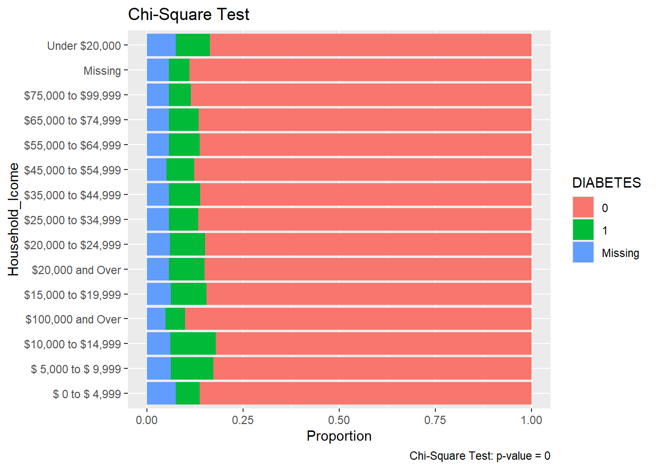
Count_Query(A_DATA_TBL_2, Grade_Level, DIABETES)
                                   Missing     0    1
Missing                               5663 59497 6681
10th grade                               9  2177   11
11th grade                               8  2146   12
12th grade, no diploma                   2   438    0
1st grade                                2  2126    6
2nd grade                                1  2102    4
3rd grade                                6  2031    6
4th grade                               12  2036    6
5th grade                               10  2110    9
6th grade                                5  2219   14
7th grade                               11  2178    8
8th grade                               12  2292   11
9th grade                               15  2195   18
High school graduate                     7  1422    9
Less than 9th grade                      1   277    1
More than high school                    3   980    6
Never attended / kindergarten only       2  2362    5
Don't Know                               0     9    0
GED or equivalent                        0   115    0
Less than 5th grade                      0    26    0
Refused                                  0     2    0
                   Missing     0    1
Missing               2548 39949 2422
$ 0 to $ 4,999         118  1349   96
$ 5,000 to $ 9,999     150  2012  268
$10,000 to $14,999     236  3169  452
$100,000 and Over      440  8226  460
$15,000 to $19,999     254  3427  375
$20,000 and Over       119  1781  194
$20,000 to $24,999     277  3902  417
$25,000 to $34,999     399  5994  526
$35,000 to $44,999     311  4738  449
$45,000 to $54,999     220  3779  311
$55,000 to $64,999     191  2878  268
$65,000 to $74,999     155  2323  205
$75,000 to $99,999     294  4580  297
Under $20,000           57   633   67
We also remark that there are some helpers for this practice if we don’t want to utilize the underlying enquo() and !! in the rlang package. This is known as the embrace operator {{}}. The embrace operator combines combines enquo() and !! in one step. For instance, out Count_Query function can be re-written as:
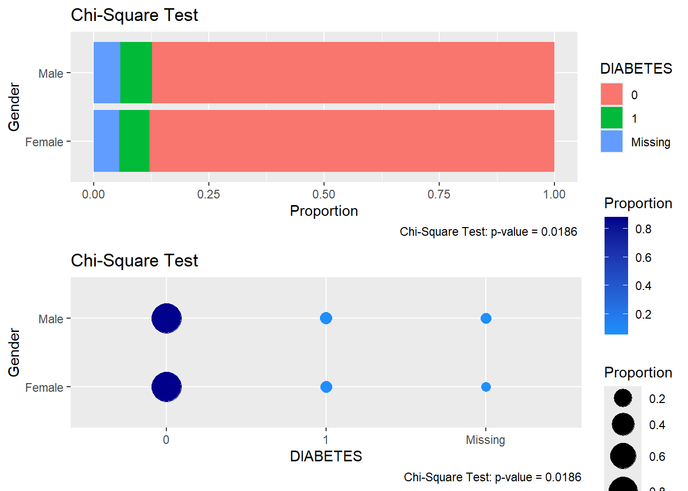
We can also make a function to display the results of the Count_Query function. This function will be a ggplot function that will display the results of the Count_Query function:
Code
plot.chisq.test.bar<-function(X){if("matrix"%in%class(X)|"table"%in%class(X)){tryCatch({X<-chisq.test(X)}, error =function(e){stop("Could not run chisq.test on the input matrix or table")})}if(class(X)!="htest"){stop("Input must be a matrix or table")}row_sums_mat<-X$observed|>rowSums()x_name<-names(dimnames(X$observed))[[1]]y_name<-names(dimnames(X$observed))[[2]]v<-as.data.frame(X$observed/row_sums_mat)|>rownames_to_column(x_name)|>tidyr::pivot_longer( cols =-all_of(x_name), names_to =y_name, values_to ='Proportion')v%>%ggplot(aes(x =Proportion, y =.data[[x_name]], fill =.data[[y_name]]))+geom_bar(stat ='identity')+labs(title ="Chi-Square Test", caption =paste0("Chi-Square Test: p-value = ", round(X$p.value, 4)))}
Previously we had the following algorithm for a t-test:
Code
## DONT RUN{dm2_age<-(A_DATA%>%filter(DIABETES==1))$Agenon_dm2_Age<-(A_DATA%>%filter(DIABETES==0))$Agett_age<-t.test(Non_DM2.Age, DM2.Age, alternative ='two.sided', conf.level =0.95)tibble_tt_age<-tt_age%>%broom::tidy()}
That process was for one t.test, for one continuous feature, Age.
We might want to functionalize the process of computing t-tests for other similar analytic data-sets, like the one we are currently working with.
Developing such functions or wrappers may take time and skill but over-time you will come to rely on a personal library of functions you develop or work with to iterate on projects faster. These functions might start in your personal library and eventually move into a team Git where you or other members of your team can manage their development.
For instance, upon inspection, we notice that t.test requires similar information to ks.test. It would make sense to bundle two tests together and save us some time later on.
8.4.1 t-test / ks-test wrapper function
In the function wrapper.t_ks_test below takes in:
df a tibble - data-frame or connection
factor a categorical variable in df
Note in SQLlite there is no factor type but the user thinks of this variable as a factor
factor_level - sets the “first” class in a one-versus-restt.test and ks.test analysis
continuous_feature represented by a character string of the feature name to perform t.test and ks.test on
verbose was useful in creating the function to identify variables causing errors, and create output for those types of cases.
You may want to put on additional safe-guards to ensure that the t.test and ks.test get valid samples, with the feature BMXRECUM we only had only 5 Diabetic member who had a non-missing value:
We will showcase how to now apply our function to every feature in our data-frame. First lets just look at the syntax for the first five numeric features: numeric_features[1:5] = PHAFSTHR, BPXML1, PHAFSTMN, BPXDI4, BPXPLS. We use the function map_dfr in the purrr library, map_dfr will attempt to return a data-frame by row-binding the results.
Below we create t_ks_result_sql with a call to map_dfr(.x, .f, ..., .id = NULL) where:
.x - A vector (numeric_features[1:5])
.f - A function (wrapper.t_ks_test)
Additional arguments passed in to the mapped function .f = wrapper.t_ks_test
df = A_DATA_TBL_2
factor = DIABETES
factor_level = 1
x the feature from the vector .x
.id - An optional character vector that will be used to name the output column of identifiers.
Each entry in numeric_features[1:5] will get passed to our function wrapper.t_ks_test produce a row like we have already seen; these rows will then be stacked together to create a data-frame.
Code
toc<-Sys.time()t_ks_result_sql<-map_dfr(numeric_features[1:5], # vector of columns (.x) \(x){# function to apply (.f)wrapper.t_ks_test( df =A_DATA_TBL_2, factor =DIABETES, factor_level =1,x# feature from the vector .x)}, .id ='Feature'# name of the output column of identifiers )# end of map_dfr
Warning in ks.test.default(X, Y): p-value will be approximate in the presence
of ties
Warning in ks.test.default(X, Y): p-value will be approximate in the presence
of ties
Warning in ks.test.default(X, Y): p-value will be approximate in the presence
of ties
Warning in ks.test.default(X, Y): p-value will be approximate in the presence
of ties
Warning in ks.test.default(X, Y): p-value will be approximate in the presence
of ties
We can see this function works, however, the SQLlight connection is slow for this kind of process, it took 14.5852031707764 seconds to perform 10 tests and get 5 result records.
Now let’s test our function here, in R, but this time we’ll use get the results for all the features:
Code
toc<-Sys.time()t_ks_result_purr<-map(numeric_features, # vector of columns \(x){wrapper.t_ks_test(# function to apply df =A_DATA_2 , factor =DIABETES , factor_level =1,x)})%>%# end of maplist_rbind(names_to ="Feature")# list_rbind turns into a data-frame
Warning in ks.test.default(X, Y): p-value will be approximate in the presence
of ties
Warning in ks.test.default(X, Y): p-value will be approximate in the presence
of ties
Warning in ks.test.default(X, Y): p-value will be approximate in the presence
of ties
Warning in ks.test.default(X, Y): p-value will be approximate in the presence
of ties
Warning in ks.test.default(X, Y): p-value will be approximate in the presence
of ties
Warning in ks.test.default(X, Y): p-value will be approximate in the presence
of ties
Warning in ks.test.default(X, Y): p-value will be approximate in the presence
of ties
Warning in ks.test.default(X, Y): p-value will be approximate in the presence
of ties
Warning in ks.test.default(X, Y): p-value will be approximate in the presence
of ties
Warning in ks.test.default(X, Y): p-value will be approximate in the presence
of ties
Warning in ks.test.default(X, Y): p-value will be approximate in the presence
of ties
Warning in ks.test.default(X, Y): p-value will be approximate in the presence
of ties
Warning in ks.test.default(X, Y): p-value will be approximate in the presence
of ties
Warning in ks.test.default(X, Y): p-value will be approximate in the presence
of ties
Warning in ks.test.default(X, Y): p-value will be approximate in the presence
of ties
Warning in ks.test.default(X, Y): p-value will be approximate in the presence
of ties
Warning in ks.test.default(X, Y): p-value will be approximate in the presence
of ties
Warning in ks.test.default(X, Y): p-value will be approximate in the presence
of ties
Warning in ks.test.default(X, Y): p-value will be approximate in the presence
of ties
Warning in ks.test.default(X, Y): p-value will be approximate in the presence
of ties
Warning in ks.test.default(X, Y): p-value will be approximate in the presence
of ties
Warning in ks.test.default(X, Y): p-value will be approximate in the presence
of ties
Warning in ks.test.default(X, Y): p-value will be approximate in the presence
of ties
Warning in ks.test.default(X, Y): p-value will be approximate in the presence
of ties
Warning in ks.test.default(X, Y): p-value will be approximate in the presence
of ties
Warning in ks.test.default(X, Y): p-value will be approximate in the presence
of ties
Warning in ks.test.default(X, Y): p-value will be approximate in the presence
of ties
Warning in ks.test.default(X, Y): p-value will be approximate in the presence
of ties
Warning in ks.test.default(X, Y): p-value will be approximate in the presence
of ties
Warning in ks.test.default(X, Y): p-value will be approximate in the presence
of ties
Warning in ks.test.default(X, Y): p-value will be approximate in the presence
of ties
Warning in ks.test.default(X, Y): p-value will be approximate in the presence
of ties
Warning in ks.test.default(X, Y): p-value will be approximate in the presence
of ties
Warning in ks.test.default(X, Y): p-value will be approximate in the presence
of ties
Warning in ks.test.default(X, Y): p-value will be approximate in the presence
of ties
Warning in ks.test.default(X, Y): p-value will be approximate in the presence
of ties
Warning in ks.test.default(X, Y): p-value will be approximate in the presence
of ties
Warning in ks.test.default(X, Y): p-value will be approximate in the presence
of ties
Warning in ks.test.default(X, Y): p-value will be approximate in the presence
of ties
Warning in ks.test.default(X, Y): p-value will be approximate in the presence
of ties
Warning in ks.test.default(X, Y): p-value will be approximate in the presence
of ties
Warning in ks.test.default(X, Y): p-value will be approximate in the presence
of ties
Warning in ks.test.default(X, Y): p-value will be approximate in the presence
of ties
Warning in ks.test.default(X, Y): p-value will be approximate in the presence
of ties
Warning in ks.test.default(X, Y): p-value will be approximate in the presence
of ties
Warning in ks.test.default(X, Y): p-value will be approximate in the presence
of ties
Warning in ks.test.default(X, Y): p-value will be approximate in the presence
of ties
Warning in ks.test.default(X, Y): p-value will be approximate in the presence
of ties
Warning in ks.test.default(X, Y): p-value will be approximate in the presence
of ties
Warning in ks.test.default(X, Y): p-value will be approximate in the presence
of ties
Warning in ks.test.default(X, Y): p-value will be approximate in the presence
of ties
Warning in ks.test.default(X, Y): p-value will be approximate in the presence
of ties
Warning in ks.test.default(X, Y): p-value will be approximate in the presence
of ties
Warning in ks.test.default(X, Y): p-value will be approximate in the presence
of ties
Warning in ks.test.default(X, Y): p-value will be approximate in the presence
of ties
Warning in ks.test.default(X, Y): p-value will be approximate in the presence
of ties
Warning in ks.test.default(X, Y): p-value will be approximate in the presence
of ties
Warning in ks.test.default(X, Y): p-value will be approximate in the presence
of ties
Warning in ks.test.default(X, Y): p-value will be approximate in the presence
of ties
Warning in ks.test.default(X, Y): p-value will be approximate in the presence
of ties
Warning in ks.test.default(X, Y): p-value will be approximate in the presence
of ties
Warning in ks.test.default(X, Y): p-value will be approximate in the presence
of ties
Warning in ks.test.default(X, Y): p-value will be approximate in the presence
of ties
Warning in ks.test.default(X, Y): p-value will be approximate in the presence
of ties
Warning in ks.test.default(X, Y): p-value will be approximate in the presence
of ties
Warning in ks.test.default(X, Y): p-value will be approximate in the presence
of ties
Warning in ks.test.default(X, Y): p-value will be approximate in the presence
of ties
Warning in ks.test.default(X, Y): p-value will be approximate in the presence
of ties
Warning in ks.test.default(X, Y): p-value will be approximate in the presence
of ties
Warning in ks.test.default(X, Y): p-value will be approximate in the presence
of ties
Warning in ks.test.default(X, Y): p-value will be approximate in the presence
of ties
Warning in ks.test.default(X, Y): p-value will be approximate in the presence
of ties
Warning in ks.test.default(X, Y): p-value will be approximate in the presence
of ties
Warning in ks.test.default(X, Y): p-value will be approximate in the presence
of ties
Warning in ks.test.default(X, Y): p-value will be approximate in the presence
of ties
Warning in ks.test.default(X, Y): p-value will be approximate in the presence
of ties
Warning in ks.test.default(X, Y): p-value will be approximate in the presence
of ties
Warning in ks.test.default(X, Y): p-value will be approximate in the presence
of ties
Warning in ks.test.default(X, Y): p-value will be approximate in the presence
of ties
Warning in ks.test.default(X, Y): p-value will be approximate in the presence
of ties
Warning in ks.test.default(X, Y): p-value will be approximate in the presence
of ties
Warning in ks.test.default(X, Y): p-value will be approximate in the presence
of ties
Warning in ks.test.default(X, Y): p-value will be approximate in the presence
of ties
Warning in ks.test.default(X, Y): p-value will be approximate in the presence
of ties
Warning in ks.test.default(X, Y): p-value will be approximate in the presence
of ties
Warning in ks.test.default(X, Y): p-value will be approximate in the presence
of ties
Warning in ks.test.default(X, Y): p-value will be approximate in the presence
of ties
Warning in ks.test.default(X, Y): p-value will be approximate in the presence
of ties
Warning in ks.test.default(X, Y): p-value will be approximate in the presence
of ties
Warning in ks.test.default(X, Y): p-value will be approximate in the presence
of ties
Warning in ks.test.default(X, Y): p-value will be approximate in the presence
of ties
Warning in ks.test.default(X, Y): p-value will be approximate in the presence
of ties
Warning in ks.test.default(X, Y): p-value will be approximate in the presence
of ties
Warning in ks.test.default(X, Y): p-value will be approximate in the presence
of ties
Warning in ks.test.default(X, Y): p-value will be approximate in the presence
of ties
Warning in ks.test.default(X, Y): p-value will be approximate in the presence
of ties
Warning in ks.test.default(X, Y): p-value will be approximate in the presence
of ties
Warning in ks.test.default(X, Y): p-value will be approximate in the presence
of ties
Warning in ks.test.default(X, Y): p-value will be approximate in the presence
of ties
Warning in ks.test.default(X, Y): p-value will be approximate in the presence
of ties
Warning in ks.test.default(X, Y): p-value will be approximate in the presence
of ties
Warning in ks.test.default(X, Y): p-value will be approximate in the presence
of ties
Warning in ks.test.default(X, Y): p-value will be approximate in the presence
of ties
Warning in ks.test.default(X, Y): p-value will be approximate in the presence
of ties
Warning in ks.test.default(X, Y): p-value will be approximate in the presence
of ties
Warning in ks.test.default(X, Y): p-value will be approximate in the presence
of ties
Warning in ks.test.default(X, Y): p-value will be approximate in the presence
of ties
Warning in ks.test.default(X, Y): p-value will be approximate in the presence
of ties
Warning in ks.test.default(X, Y): p-value will be approximate in the presence
of ties
Warning in ks.test.default(X, Y): p-value will be approximate in the presence
of ties
Warning in ks.test.default(X, Y): p-value will be approximate in the presence
of ties
Warning in ks.test.default(X, Y): p-value will be approximate in the presence
of ties
Warning in ks.test.default(X, Y): p-value will be approximate in the presence
of ties
Warning in ks.test.default(X, Y): p-value will be approximate in the presence
of ties
Warning in ks.test.default(X, Y): p-value will be approximate in the presence
of ties
Warning in ks.test.default(X, Y): p-value will be approximate in the presence
of ties
Warning in ks.test.default(X, Y): p-value will be approximate in the presence
of ties
Warning in ks.test.default(X, Y): p-value will be approximate in the presence
of ties
Warning in ks.test.default(X, Y): p-value will be approximate in the presence
of ties
Warning in ks.test.default(X, Y): p-value will be approximate in the presence
of ties
Warning in ks.test.default(X, Y): p-value will be approximate in the presence
of ties
Warning in ks.test.default(X, Y): p-value will be approximate in the presence
of ties
Warning in ks.test.default(X, Y): p-value will be approximate in the presence
of ties
Warning in ks.test.default(X, Y): p-value will be approximate in the presence
of ties
Warning in ks.test.default(X, Y): p-value will be approximate in the presence
of ties
Warning in ks.test.default(X, Y): p-value will be approximate in the presence
of ties
Warning in ks.test.default(X, Y): p-value will be approximate in the presence
of ties
Warning in ks.test.default(X, Y): p-value will be approximate in the presence
of ties
Warning in ks.test.default(X, Y): p-value will be approximate in the presence
of ties
Warning in ks.test.default(X, Y): p-value will be approximate in the presence
of ties
Warning in ks.test.default(X, Y): p-value will be approximate in the presence
of ties
Warning in ks.test.default(X, Y): p-value will be approximate in the presence
of ties
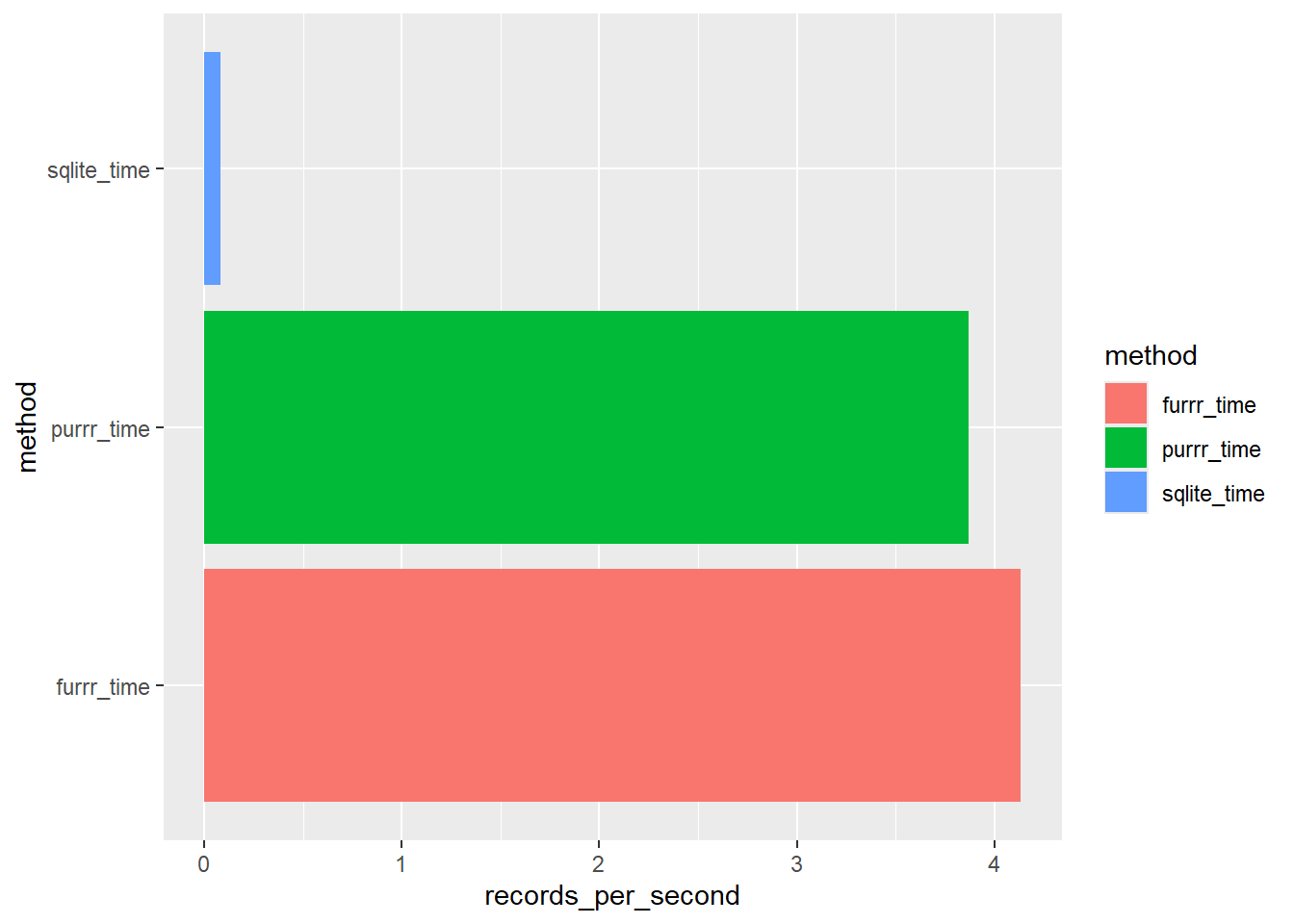
We have already mentioned that these results are confined to our SQLite connection. In some cases, you might be able to write a t-test / ks-test wrapper that performs better when computed on a server rather than within a local R session.
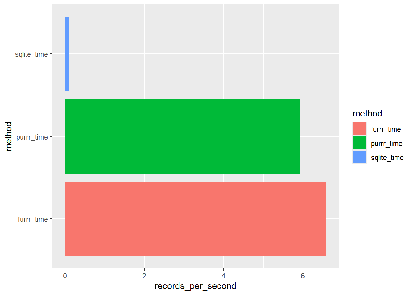
8.7 Compairing Outputs
The arsenal package contains a handy function comparedf to compare two data-frames. We can see that t_ks_result_purr and t_ks_result_furr match:
Compare Object

Function Call:
arsenal::comparedf(x = t_ks_result_purr, y = t_ks_result_furr)

Shared: 14 non-by variables and 67 observations.
Not shared: 1 variables and 0 observations.

Differences found in 0/14 variables compared.
0 variables compared have non-identical attributes.
However, t_ks_result_sql and t_ks_result_purr do not:
Compare Object

Function Call:
arsenal::comparedf(x = t_ks_result_purr, y = t_ks_result_sql)

Shared: 15 non-by variables and 5 observations.
Not shared: 0 variables and 62 observations.

Differences found in 0/15 variables compared.
0 variables compared have non-identical attributes.
List of 9
 $ frame.summary.table     :'data.frame':   2 obs. of  4 variables:
 $ comparison.summary.table:'data.frame':   13 obs. of  2 variables:
 $ vars.ns.table           :'data.frame':   0 obs. of  4 variables:
 $ vars.nc.table           :'data.frame':   0 obs. of  6 variables:
 $ obs.table               :'data.frame':   62 obs. of  3 variables:
 $ diffs.byvar.table       :'data.frame':   15 obs. of  4 variables:
 $ diffs.table             :'data.frame':   0 obs. of  7 variables:
 $ attrs.table             :'data.frame':   0 obs. of  3 variables:
 $ control                 :List of 16
 - attr(*, "class")= chr "summary.comparedf"
this is the comparison.summary.table
Code
compare.details$comparison.summary.table
                                                     statistic value
1                                       Number of by-variables     0
2                         Number of non-by variables in common    15
3                                 Number of variables compared    15
4                           Number of variables in x but not y     0
5                           Number of variables in y but not x     0
6        Number of variables compared with some values unequal     0
7           Number of variables compared with all values equal    15
8                             Number of observations in common     5
9                        Number of observations in x but not y    62
10                       Number of observations in y but not x     0
11 Number of observations with some compared variables unequal     0
12    Number of observations with all compared variables equal     5
13                                    Number of values unequal     0
for instance compare.details$obs.table has the elements in t_ks_result_purr (x) that are not within t_ks_result_sql (y):
# Functional dbplyr, purrr, and furrr {#sec-functional-dbplyr-purrr-and-furrr}```{r}#| label: 4-1-tidyverse #| cache: falselibrary('tidyverse')source(here::here('Functions/connect_help.R'))```#### `source` current target```{r}#| label: 4-1-source-target #| cache: falsesource(here::here("DATA/Part_4/FEATURES/Store_TARGET_DM2.R"))```#### `source` current features```{r}#| label: 4-1-source-features#| cache: false source(here::here('DATA/Part_4/FEATURES/Store_DEMO.R'))source(here::here('DATA/Part_4/FEATURES/Store_EXAM.R'))source(here::here('DATA/Part_4/FEATURES/Store_LABS.R'))```### `A_DATA_TBL_2`We want to make a new Analytic data-set from additional features that have been developed. We might begin to cultivate a **Feature Store** which might comprise of either code or data to replicate features.```{r}#| label: 4-1-A-Data-TBL-2#| cache: false A_DATA_TBL_2 <- DEMO %>%select(SEQN) %>%left_join(OUTCOME_TBL) %>%left_join(DEMO_FEATURES) %>%left_join(EXAM_TBL) %>%left_join(LABS_TBL)```Get the dimension from a connection```{r}#| label: 4-1-row-connection#| cache: false nrow.table <-function(con_tbl){# number of rows Tot_N_Rows <- con_tbl %>%summarise(n =n()) %>%pull(n) Tot_N_Rows}nrow.table(A_DATA_TBL_2)``````{r}#| error: TRUETot_N_Rows``````{r}#| label: 4-1-dim-connection#| cache: false dim.table <-function(con_tbl){# number of rows Tot_N_Rows <-nrow.table(con_tbl) # number of columns Tot_N_Cols <- tbl %>%colnames() %>%length() result <-c(Tot_N_Rows, Tot_N_Cols) result} dim.table(A_DATA_TBL_2) ``````{r}Tot_N_Rows <-nrow.table(A_DATA_TBL_2)``````{r}#| label: 4-1-glimpse-1#| cache: false#look at the data-set A_DATA_TBL_2 %>%head()```## Determining Categorical and Continuous Features```{r}#| label: 4-1-Not-features#| cache: falseNot_features <-c('SEQN', 'DIABETES', 'AGE_AT_DIAG_DM2')All_featres <-setdiff(colnames(A_DATA_TBL_2), Not_features)``````{r}#| label: 4-1-n-levels-featuress#| cache: falseN_levels_features <- A_DATA_TBL_2 %>%select(-all_of(Not_features)) %>%summarise(across(all_of(All_featres), \(x){n_distinct(x)} ) ) %>%collect() # note this collects all the dataN_levels_features %>%head()``````{r}#| label: 4-1-pivot-n-levels-features#| cache: falseN_levels_features %>%pivot_longer( cols =all_of(All_featres), values_to ="N_Distinct_Values") %>%arrange(desc(N_Distinct_Values))``````{r}#| label: 4-1-n-levels-1#| cache: false#| fig-cap: "Count of Distinct Number of Values Per Feature" N_levels_features %>%pivot_longer( cols =all_of(All_featres), values_to ="N_Distinct_Values") %>%mutate(Fearure =reorder(name, -N_Distinct_Values)) %>%mutate(Percentage_Distinct_Features = N_Distinct_Values/Tot_N_Rows ) %>%ggplot(aes(x= Fearure, y=Percentage_Distinct_Features , fill=Percentage_Distinct_Features)) +geom_bar(stat ="identity") +coord_flip() +theme(legend.position ="none") ``````{r}#| label: 4-1-features-with-15-to-70-levels#| cache: falseN_levels_features %>%pivot_longer( cols =all_of(All_featres), values_to ="N_Distinct_Values") %>%arrange(N_Distinct_Values) %>%filter(15< N_Distinct_Values & N_Distinct_Values <70)``````{r}#| label: 4-1-categorical_features#| cache: falsecategorical_features <- N_levels_features %>%pivot_longer( cols =all_of(All_featres), values_to ="N_Distinct_Values") %>%arrange(N_Distinct_Values) %>%filter(N_Distinct_Values <=25) %>%pull(name)names(categorical_features) <- categorical_featurescategorical_features```Currently, there are `r length(categorical_features)` and```{r}#| label: 4-1-numeric_featuress#| cache: falsenumeric_features <- N_levels_features %>%pivot_longer( cols =all_of(All_featres), values_to ="N_Distinct_Values") %>%arrange(N_Distinct_Values) %>%filter(N_Distinct_Values >25) %>%pull(name)names(numeric_features) <- numeric_features numeric_features```we have `r length(numeric_features)` numeric features to analyze.We can save both of these lists into an new object:```{r}#| label: 4-1-FEATURE_TYPE #| cache: falsenames(Not_features) <- Not_featuresFEATURE_TYPE <-new.env()FEATURE_TYPE$numeric_features <- numeric_featuresFEATURE_TYPE$categorical_features <- categorical_featuresFEATURE_TYPE$Not_features <- Not_features```We can still access the information, however, now it is grouped together:```{r}#| label: 4-1-cat-1 #| cache: falseFEATURE_TYPE$categorical_features``````{r , cache=FALSE}#| label: 4-1-cont#| cache: falseFEATURE_TYPE[['numeric_features']]```### distinct_N_levels_per_cols Below is a helper function for the count of distinct column entries in a table per the first `sample_n` records queried ```{r}#| label: 4-1-dis-N-levels-fun#| cache: falsedistinct_N_levels_per_cols <-function(data){ data.colnames <-colnames(data) N_levels_features <- data %>%summarise(across(all_of(data.colnames), \(x){n_distinct(x)}) ) %>%collect() %>%pivot_longer( cols =all_of(data.colnames), values_to ="N_Distinct_Values") plot <- N_levels_features %>%mutate(Fearure =reorder(name, -N_Distinct_Values)) %>%mutate(Percentage_Distinct_Features = N_Distinct_Values/nrow.table(data)) %>%ggplot(aes(x= Fearure, y=Percentage_Distinct_Features , fill=Percentage_Distinct_Features)) +geom_bar(stat ="identity") +coord_flip() +labs(title ="Percentage of Distinct Entries Per Column") +theme(legend.position ="none")return( list( data = N_levels_features,plot = plot))}``````{r}#| label: fig-4-1-dis-N-levels-ex-3241#| cache: false#| fig-cap: "Count of Distinct Number of Values Per Feature records"distinct_N_levels_per_cols(A_DATA_TBL_2)$plot```## Categorical FeaturesRecall, we normally want to review categorical data by looking at frequency counts:```{r}#| label: 4-1-DM2-Gender-tally#| cache: false A_DATA_TBL_2 %>%select(DIABETES, Gender) %>%group_by(DIABETES, Gender) %>%tally() %>%collect() %>%ungroup() %>%mutate(across(c("DIABETES", "Gender"), \(x){as.character(x)} ) ) %>%mutate(across(c("DIABETES", "Gender"), \(x){if_else(is.na(x), "Missing", x)} ) ) %>%pivot_wider(names_from = DIABETES, values_from = n)``````{r}#| label: 4-1-DM2-Race-tally-t #| cache: falseA_DATA_TBL_2 %>%select(DIABETES, Race) %>%group_by(DIABETES, Race) %>%tally() %>%collect() %>%ungroup() %>%mutate(across(c("DIABETES", "Race"), \(x){as.character(x)} ) ) %>%mutate(across(c("DIABETES", "Race"), \(x){if_else(is.na(x), "Missing", x)} ) ) %>%pivot_wider(names_from = DIABETES, values_from = n)```### `Count_Query` functionSo to functionalize this process we create the following:```{r}#| label: 4-1-count-query-function #| cache: falseCount_Query <-function(data, my_feature, outcome){ enquo_feature <-enquo(my_feature) enquo_outcome <-enquo(outcome) tmp <- data %>%select(!!enquo_outcome, !!enquo_feature) %>%group_by(!!enquo_outcome, !!enquo_feature) %>%tally() %>%collect() %>%ungroup() %>%mutate(across(c(!!enquo_outcome, !!enquo_feature), \(x){as.character(x)} ) ) %>%mutate(across(c(!!enquo_outcome, !!enquo_feature), \(x){if_else(is.na(x), "Missing", x)} ) ) %>%pivot_wider(names_from =!!enquo_outcome, values_from = n,values_fill =0)row_names <-if_else(is.na(tmp[[1]]),"NA", tmp[[1]]) tmp <- tmp[-1]matrix_tmp <-as.matrix(tmp)row.names(matrix_tmp) <- row_namesreturn(matrix_tmp)}```What is `enquo`?`enquo()` and `enquos()` delay the execution of one or several function arguments. `enquo()` returns a single quoted expression, which is like a blueprint for the delayed computation. `enquos()` returns a list of such quoted expressions. We can resolve an `enquo` with `!!`.```{r}#| label: 4-1-count-query-grade #| cache: falseCount_Query(A_DATA_TBL_2, Grade_Level, DIABETES) ``````{r}#| label: 4-1-count-query-household Count_Query(A_DATA_TBL_2, Household_Icome, DIABETES)```We also remark that there are some helpers for this practice if we don't want to utilize the underlying `enquo()` and `!!` in the `rlang` package. This is known as the embrace operator `{{}}`. The embrace operator combines combines `enquo()` and `!!` in one step. For instance, out `Count_Query` function can be re-written as: ```{r}Count_Query <-function(data, my_feature, outcome){ my_feature_car <- data %>%select({{my_feature}}) |>colnames() my_outcome_car <- data %>%select({{outcome}}) |>colnames() tmp <- data %>%select({{outcome}}, {{my_feature}}) %>%group_by({{outcome}}, {{my_feature}}) %>%tally() %>%collect() %>%ungroup() %>%mutate(across(c({{outcome}}, {{my_feature}}), \(x){as.character(x)} ) ) %>%mutate(across(c({{outcome}}, {{my_feature}}), \(x){if_else(is.na(x), "Missing", x)} ) ) %>%pivot_wider(names_from = {{outcome}}, values_from = n,values_fill =0)row_names <-if_else(is.na(tmp[[1]]),"NA", tmp[[1]]) tmp <- tmp[-1]matrix_tmp <-as.matrix(tmp)row.names(matrix_tmp) <- row_namesdimnames(matrix_tmp) <-list(row_names, colnames(matrix_tmp))names(dimnames(matrix_tmp)) <-c(my_feature_car, my_outcome_car)return(matrix_tmp)}```### Graphing HelpersWe can also make a function to display the results of the `Count_Query` function. This function will be a `ggplot` function that will display the results of the `Count_Query` function:```{r}#| label: 4-1-count-query-grade-fun #| cache: falseplot.chisq.test.bar <-function(X){if("matrix"%in%class(X) |"table"%in%class(X)){tryCatch({ X <-chisq.test(X) }, error =function(e) {stop("Could not run chisq.test on the input matrix or table") }) }if(class(X) !="htest"){stop("Input must be a matrix or table") } row_sums_mat <- X$observed |>rowSums() x_name <-names(dimnames(X$observed))[[1]] y_name <-names(dimnames(X$observed))[[2]] v <-as.data.frame(X$observed/row_sums_mat) |>rownames_to_column(x_name) |> tidyr::pivot_longer(cols =-all_of(x_name),names_to = y_name, values_to ='Proportion') v %>%ggplot(aes(x = Proportion, y = .data[[x_name]], fill = .data[[y_name]])) +geom_bar(stat ='identity') +labs(title ="Chi-Square Test",caption =paste0("Chi-Square Test: p-value = ", round(X$p.value, 4))) }``````{r}#| label: 4-1-chi-square-grade-level#| cache: false#| fig-cap: "Chi-Square - Grade Level by Diabetes"Count_Query(A_DATA_TBL_2, Household_Icome, DIABETES) |>plot.chisq.test.bar()```Or a function to help us with balloon plots:```{r}#| label: 4-1-balloon-plot-helper#| cache: falseplot.chisq.test.balloon <-function(X){if("matrix"%in%class(X) |"table"%in%class(X)){tryCatch({ X <-chisq.test(X) }, error =function(e) {stop("Could not run chisq.test on the input matrix or table") }) }if(class(X) !="htest"){stop("Input must be a matrix or table") } row_sums_mat <- X$observed |>rowSums() x_name <-names(dimnames(X$observed))[[1]] y_name <-names(dimnames(X$observed))[[2]] v <-as.data.frame(X$observed/row_sums_mat) |>rownames_to_column(x_name) |> tidyr::pivot_longer(cols =-all_of(x_name),names_to = y_name, values_to ='Proportion') v %>%ggplot(aes(x = .data[[y_name]], y = .data[[x_name]], size = Proportion, color=Proportion)) +geom_point() +scale_size_continuous(range =c(3, 10)) +scale_color_gradient(low ="dodgerblue", high ="darkblue") +labs(title ="Chi-Square Test",caption =paste0("Chi-Square Test: p-value = ", round(X$p.value, 4)))}``````{r}Count_Query(A_DATA_TBL_2, Household_Icome, DIABETES) |>plot.chisq.test.balloon() ```#### Combine functions to create new functionsWe can combine functions:```{r}#| label: 4-1-combine-functions plot.chisq.test <-function(X, method){if(method =='bar'){return(plot.chisq.test.bar(X)) }if(method =='balloon'){return(plot.chisq.test.balloon(X)) }if(method =='both'){return( gridExtra::grid.arrange(plot.chisq.test.bar(X), plot.chisq.test.balloon(X), nrow =2)) }}``````{r}#| label: 4-1-combine-plot-Gender#| fig-cap: "Combine Plots Gender"Count_Query(A_DATA_TBL_2, Gender, DIABETES) %>%plot.chisq.test(method ='both') ```## Additional Programming Refrences- <https://rlang.r-lib.org/reference/embrace-operator.html>- <https://dplyr.tidyverse.org/articles/programming.html#indirection-1>## Continuous FeaturesPreviously we had the following algorithm for a t-test:```{r}#| label: 4-1-previous_ttest#| eval: false## DONT RUN{dm2_age <- (A_DATA %>%filter(DIABETES ==1))$Agenon_dm2_Age <- (A_DATA %>%filter(DIABETES ==0))$Agett_age <-t.test(Non_DM2.Age, DM2.Age, alternative ='two.sided', conf.level =0.95)tibble_tt_age <- tt_age %>% broom::tidy()}```That process was for one `t.test`, for one continuous feature, `Age`.We might want to functionalize the process of computing t-tests for other similar analytic data-sets, like the one we are currently working with.Developing such functions or wrappers may take time and skill but over-time you will come to rely on a personal library of functions you develop or work with to iterate on projects faster. These functions might start in your personal library and eventually move into a team Git where you or other members of your team can manage their development.For instance, upon inspection, we notice that `t.test` requires similar information to `ks.test`. It would make sense to bundle two tests together and save us some time later on.### t-test / ks-test wrapper functionIn the function `wrapper.t_ks_test` below takes in:1. `df` a tibble - data-frame or connection2. `factor` a categorical variable in df - Note in SQLlite there is no factor type but the user thinks of this variable as a factor3. `factor_level` - sets the **"first"** class in a **one-versus-rest** `t.test` and `ks.test` analysis4. `continuous_feature` represented by a character string of the feature name to perform `t.test` and `ks.test` on5. `verbose` was useful in creating the function to identify variables causing errors, and create output for those types of cases.```{r}#| label: 4-1-wrapper-t-ks-test#| cache: false wrapper.t_ks_test <-function(df, factor, factor_level, continuous_feature, verbose =FALSE){if(verbose ==TRUE){cat(paste0('\n','Now on Feature ',continuous_feature,' \n')) } data.local <- df %>%select({{factor}}, matches(continuous_feature)) %>%collect() X <- data.local %>%filter({{factor}} == factor_level) %>%pull(continuous_feature) Y <- data.local %>%filter({{factor}} != factor_level) %>%pull(continuous_feature) sd_x <-sd(X, na.rm=TRUE) sd_y <-sd(Y, na.rm=TRUE)if(sum(!is.na(X)) <3|sum(!is.na(Y)) <3|is.na(sd_x) |is.na(sd_y) | sd_x ==0| sd_y ==0){ err_return <-tibble(estimate1 =mean(X, na.rm =TRUE),estimate2 =mean(Y, na.rm =TRUE),N_Target =sum(!is.na(X)),N_Control =sum(!is.na(Y)) ) %>%mutate(estimate = estimate1 - estimate2)return(err_return) } test_result <-t.test(X,Y) %>% broom::tidy() %>%rename(ttest.pvalue = p.value) %>%rename(t.statistic = statistic) kstest_result <-ks.test(X,Y) %>% broom::tidy() %>%rename(kstest.pvalue = p.value) %>%rename(ks.statistic = statistic) %>%select(kstest.pvalue, ks.statistic) result <-cbind(test_result, kstest_result) %>%mutate(N_Target =sum(!is.na(X))) %>%mutate(N_Control =sum(!is.na(Y))) return(result)if(verbose ==TRUE){cat(paste0('\n','Finished Feature ',continuous_feature,' \n')) }}```### Test FunctionNow we can test our function:```{r}#| label: 4-1-wrapper-t_ks_test-Agewrapper.t_ks_test(df=A_DATA_TBL_2 , factor = DIABETES, factor_level =1, 'Age') %>%select(-where(is.character)) %>%pivot_longer(everything(),names_to ='Test',values_to ='Value')```You may want to put on additional safe-guards to ensure that the `t.test` and `ks.test` get valid samples, with the feature `BMXRECUM` we only had only `r wrapper.t_ks_test(df=A_DATA_TBL_2 , factor = DIABETES , factor_level = 1, 'BMXRECUM')$N_Target` Diabetic member who had a non-missing value:```{r}#| label: 4-1-wrapper-t_ks_test-BMXRECUM wrapper.t_ks_test(df = A_DATA_TBL_2 , factor = DIABETES , factor_level =1, 'BMXRECUM') %>%glimpse()```## `purrr`We will showcase how to now apply our function to every feature in our data-frame. First lets just look at the syntax for the first five numeric features: `numeric_features[1:5] =``r numeric_features[1:5]`. We use the function `map_dfr` in the `purrr` library, `map_dfr` will attempt to return a data-frame by row-binding the results.Below we create `t_ks_result_sql` with a call to `map_dfr(.x, .f, ..., .id = NULL)` where:- `.x` - A vector (`numeric_features[1:5]`)- `.f` - A function (`wrapper.t_ks_test`) - Additional arguments passed in to the mapped function `.f = wrapper.t_ks_test` - `df = A_DATA_TBL_2` - `factor = DIABETES` - `factor_level = 1` - `x` the feature from the vector `.x`- `.id` - An optional character vector that will be used to name the output column of identifiers. Each entry in `numeric_features[1:5]` will get passed to our function `wrapper.t_ks_test` produce a row like we have already seen; these rows will then be stacked together to create a data-frame.```{r}#| label: 4-1-A_DATA_TBL_2.t_ks_result.sq toc <-Sys.time()t_ks_result_sql <-map_dfr( numeric_features[1:5], # vector of columns (.x) \(x){ # function to apply (.f)wrapper.t_ks_test(df = A_DATA_TBL_2,factor = DIABETES,factor_level =1, x# feature from the vector .x )},.id ='Feature'# name of the output column of identifiers ) # end of map_dfrtic <-Sys.time()sql_con_time <-difftime(tic, toc, units='secs')sql_con_time```We can see this function works, however, the SQLlight connection is slow for this kind of process, it took `r sql_con_time` seconds to perform `r 2*nrow(t_ks_result_sql)` tests and get `r nrow(t_ks_result_sql)` result records.We might try to download the data:```{r}#| label: 4-1-A_DATA_2toc <-Sys.time()A_DATA_2 <- A_DATA_TBL_2 %>%collect()tic <-Sys.time()download_time <-difftime(tic , toc, units='secs')``````{r 4-1-download-time }download_time```How large is `A_DATA_2` ?```{r}#| label: 4-1-dim-local dim(A_DATA_2)format(object.size(A_DATA_2),"Mb")```Now let's test our function here, in `R`, but this time we'll use get the results for all the features:```{r}#| label: 4-1-A_DATA_TBL_2.t_ks_result.purrr4 toc <-Sys.time()t_ks_result_purr <-map( numeric_features, # vector of columns \(x){wrapper.t_ks_test( # function to applydf = A_DATA_2 , factor = DIABETES , factor_level =1, x)} ) %>%# end of maplist_rbind(names_to ="Feature") # list_rbind turns into a data-frametic <-Sys.time()local_time <-difftime(tic , toc , units='secs')``````{r}#| label: 4-1-local-time local_time``````{r}#| label: 4-1-speed-purr-sql as.numeric(local_time) /as.numeric(sql_con_time)```That's quite a speed-up to get all `r nrow(t_ks_result_purr)` results in `r local_time` seconds but we can most likely do even better with the `furrr` package:## `furrr````{r}#| label: 4-1-furrr library('furrr')no_cores <-availableCores() no_coresfuture::plan(multicore, workers = no_cores)``````{r}#| label: 4-1-furrr_test toc <-Sys.time()t_ks_result_furr <- furrr::future_map_dfr( numeric_features, # vector of columns function(x){wrapper.t_ks_test(df=A_DATA_2 ,factor = DIABETES ,factor_level =1, x) })tic <-Sys.time()furrr_time <- tic - toc```### Compare Run Times```{r}#| label: 4-1-compare-timessql_v_purrr_v_furrr <-bind_rows(tibble(time = sql_con_time , n_records =nrow(t_ks_result_sql), method ='sqlite_time'),tibble(time = local_time , n_records =nrow(t_ks_result_purr), method ='purrr_time'),tibble(time = furrr_time , n_records =nrow(t_ks_result_purr), method ='furrr_time')) %>%mutate(records_per_second = n_records/as.double(time)) ``````{r}#} label: 4-1-load-manual-run#| echo: falsesql_v_purrr_v_furrr <-readRDS(here::here("DATA/Part_4/sql_v_purrr_v_furrr.RDS"))``````{r}#| label: 4-1-compare-times-graph sql_v_purrr_v_furrr %>%ggplot(aes(x= method, y=records_per_second, fill=method)) +geom_bar(stat ="identity", position=position_dodge()) +coord_flip()sql_v_purrr_v_furrr```Even accounting for download times we can see that does not have much of an effect:```{r}#| label: 4-1-sql-purrr-furrr #| fig-cap: "Time comparison" sql_v_purrr_v_furrr %>%mutate(download_time = download_time) %>%mutate(time_plus_download =if_else( method !='sqlite_time', time + download_time, time)) %>%mutate(records_per_second = n_records/as.numeric(time_plus_download)) %>%ggplot(aes(x= method, y=records_per_second, fill=method)) +geom_bar(stat ="identity", position=position_dodge()) +coord_flip()``````{r}#| label: 4-1-rps#| fig-cap: "Records Per Second SQLite Vs purrr Vs furrr"records_per_second_plus_download <- sql_v_purrr_v_furrr %>%mutate(download_time = download_time) %>%mutate(time_plus_download =if_else( method !='sqlite_time', time + download_time, time)) %>%mutate(records_per_second = n_records/as.numeric(time_plus_download)) %>%select(method, records_per_second) %>%pivot_wider(names_from = method, values_from = records_per_second)records_per_second_plus_download```Even accounting for download speeds locally with `purrr` our function is```{r}#| label: 4-1-rps-2records_per_second_plus_download$purrr_time / records_per_second_plus_download$sqlite_time ```times faster than with our SQLite connection and in this case `furrr` is ```{r}#| label: 4-1-rps-3records_per_second_plus_download$furrr_time / records_per_second_plus_download$purrr_time ```times faster than `purrr`.#### Results Vary By Connection TypeWe have already mentioned that these results are confined to our SQLite connection. In some cases, you might be able to write a t-test / ks-test wrapper that performs better when computed on a server rather than within a local `R` session. ## Compairing OutputsThe `arsenal` package contains a handy function `comparedf` to compare two data-frames. We can see that `t_ks_result_purr` and `t_ks_result_furr` match:```{r}#| label: 4-1-arsenal-1arsenal::comparedf(t_ks_result_purr, t_ks_result_furr)```However, `t_ks_result_sql` and `t_ks_result_purr` do not:```{r}#| label: 4-1-arsenal-2arsenal::comparedf(t_ks_result_purr, t_ks_result_sql)```we can get a detailed summary of the outputs```{r}#| label: 4-1-arsenal-3compare.details <- arsenal::comparedf(t_ks_result_purr, t_ks_result_sql) %>%summary()```there are several tables to review```{r}str(compare.details,1)```this is the `comparison.summary.table````{r}#| label: 4-1-sum-arsenal-1compare.details$comparison.summary.table```for instance `compare.details$obs.table` has the elements in `t_ks_result_purr` (`x`) that are not within `t_ks_result_sql` (`y`):```{r}#| label: 4-1-sum-arsenal-2compare.details$obs.table %>%head()```If we want the top 10 corresponding records we could do:```{r}#| label: 4-1-sum-arsenal-3t_ks_result_purr[compare.details$obs.table$observation[1:10],] %>%select(Feature, ttest.pvalue, kstest.pvalue) %>% knitr::kable()```## Disscussion> How do the functions Count_Query, wrapper.t_ks_test, and logit_model_scorer from last chapter compare?#### Save Data```{r save-data}A_DATA_2 %>% saveRDS(here::here('DATA/Part_4/A_DATA_2.RDS'))t_ks_result_furr %>% saveRDS(here::here('DATA/Part_4/t_ks_result_furr.RDS'))FEATURE_TYPE %>% saveRDS(here::here('DATA/Part_4/FEATURE_TYPE.RDS'))``````{r save-data2 , echo=FALSE}A_DATA_2 %>% saveRDS(here::here('DATA/Part_5/A_DATA.RDS'))t_ks_result_furr %>% saveRDS(here::here('DATA/Part_5/t_ks_result_furr.RDS'))``````{r}DBI::dbDisconnect(NHANES_DB)```