Time Series and Random Forest
Conceptual Framework Of Time Series Analysis
Data having date and time features can be modeled in two ways depending upon whether the dates and times are collected within subject or across subject. Data with dates and times collected within subject are often analyzed as a time series as the these subjects are tracked with consecutive dates and times beginning with a start time and an end time. These time series data are then dependent upon sequences of time. When the data are collected on subjects without regard to within subject time tagging, the analysis uses dates and times as independent features rather than time dependent features.
Many disciplines such as medicine, economics, the social sciences, and the physical sciences; collect data as a function of time. The collection periods may be seconds, hours, days, weeks, months, or years, for a few examples. Stock traders may collect second-by-second data, whereas, human birthrates are often collected as the number per day. A long standing monthly data collection endeavor is the number of Sunspots. Finally, climate data such as temperature changes are recorded annually. Each of these examples is a collection of data indexed on time, and models often are constructed to better understand the time-based structure or to forecast future events.
The general purpose of time series modeling is understand fluctuations in data as a function of time and, in some cases, also a function of time-varying or non-time-varying covariates. The fluctuations may be short term, i.e., they have a short term memory, or they may be long term fluctuations having thereby a long term memory. The fluctuations may appear to be random, they may have a linear or nonlinear trend, or they may be cyclical such as having a seasonal component.
White noise is an example of random fluctuations through time. White noise is characterized by identically independently distributed random variables indexed by time of occurrence. If the unexplained variation resulting from a time series model is white noise, we say the model is an adequate fit to the data from which it was constructed.
Trends in time series data may be linear or nonlinear. They may have a positive (increasing) growth pattern, they may have a negative (decreasing) pattern, or there may be multiple trends, both positive and negative, embedded in the series. A time series model must account for trends to provide and unbiased fit and accurate forecasts.
Seasons in time series data are patterns that cycle in time. These cycles may be sinusoidal, sawtooth, or square, among a number of other possible shapes. The periods may be short, e.g., seconds, or long, e.g., decades. Time series models, as with trends, must account for cycling in the data, including multiple seasonal cycle periods. It is not uncommon to have time series data with both trends and seasons.
Because time series data may have any combination of random fluctuations, trends, and seasons, two possible approaches for modeling time series data have historical development. The approaches are models for the time domain and models for the frequency domain.
Time domain analyses derive from the correlation structure between adjacent time values and can be modeled by a weighted regression of the current value on past values. This is possible from the assumption that the current value can be predicted by the sum of a linear combination of the past values of a noise component and a deterministic component orthogonal to the linear noise sum. Thus, we partition the data into a component whose variation is accounted for by the past values, and a component whose variation is completely random. The time domain modeling method estimates the regression coefficients as well as determining the number of these coefficients. The estimation method varies according to the properties of the time series data and the intent of the analyst. Some estimation methods include ordinary least squares, maximum likelihood, and bayesian estimation. Time domain analyses are ubiquitous across disciplines.
Typical time domain models include autoregressive integrated moving average models, seasonal autoregressive moving average models, autoregressive conditionally heteroscedastic and generalized autoregressive conditionally heteroscedastic volatility models, smoothing models such as exponential smoothing and X11, and hidden Markov models. Often time domain data are modeled by generalized additive models such as is used by Facebook (Taylor SJ 2017 [Online]). Details of these and other models may be found in these texts: Pfaff (2008); and (Tsay 2010).
The frequency domain modeling method assumes that the time series is best described by a sum or a linear superposition of periodic sine and cosine waves of different periods (frequencies). A spectral representation of a stationary time series may be constructed from the superposition giving parameters and power plots that reveal the strong components from weaker components, and from noise. Frequency domain analyses are common in the physical sciences.
Some popular frequency domain analytical methods are Fourier series, Fourier transforms, Laplace transforms, Z transforms, and wavelet transforms. Fourier series are linear combinations of sine and cosine wave functions of differing frequencies. Fourier transformations allow for non-periodic functions in addition to periodic functions. The Laplace transform converts real-valued time series into complex-valued time series. The Z transform converts a discrete time series into a complex-valued time series. Wavelet transforms allow for the integration of the frequency domain with the time domain at high frequencies. More information on these models is in these texts: Nason (2008); and (Shumway 1988).
Both time domain and frequency domain data may be modeled by machine learning algorithms. The algorithms include recurrent neural networks and ensemble learning based on decision trees. Recurrent neural networks use a feedback and/or feedforward networks using impulse or frequency response functions. Random forest analysis consists of generating multiple decision trees from randomly modified tree node decision values and randomly selected features (variables). The aggregation of the resulting trees produces a class of decision values and features most often selected by the multiplicity of trees. Further reading on neural networks may be found in Chollet (2021); and (Mehlig 2021).
The primary objective of time series analysis is to develop mathematical models that provide sufficient descriptions of the sample data. Time series data are considered to be a collection of random variables such that for all time-indexed random variables, \(X_t, \ t = 1, \ldots, T\). Although the \(X_t\) may be continuous, we treat the samples as discrete with, often, equally separated time increments. Equal separation is not mandatory with all time series models, however. We describe in more detail below, how random forest analysis is conducted.
Random Forest Time Series Analysis
We now describe random forest time series analysis. We begin with a description of decision trees and then turn to the use of decision trees in random forest analysis. Unlike a random forest analysis of data not dependent upon time, random forest analysis for time series must accommodate time sequenced data, most likely with an autocorrelation structure. Standard implementations of random forest analysis consider the data to have independent observations. One method for accommodating the autocorrelation structure is to use a sliding window technique. Other methods, are the non-overlapping block bootstrap, the moving block bootstrap, and the circular block bootstrap.
Sliding Window
The sliding window technique assumes a predetermined autocorrelation structure. As an example, the simplest autocorrelation structure is one in which the current observation is predicted by its immediate predecessor; viz., for a time series indexed by the integers \(\mathbb{Z}^* = \{1, 2, \ldots, T\}\), the \(t\)th observation is a linear function of the \((t-1)\)th observation, \(X_t = \phi_1 X_{t-1}, \ t \in \mathbb{Z}^*\). This model is known as an Autoregressive model of order 1, denoted AR(1). The AR(1) model is said to be autocorrelated at lag 1, where lag 1 is the \(t-1\)st observation for all \(t \in \{2, 3,\ldots,T\}\).
The AR(1) model is implemented for random forest analysis by shifting the original time series forward one time interval such that one column of the data matrix is the original time series with an NA in the first row (\(t=1\)) and the second row has the \(t=1\) observation of the time series, row 3 is the \(t=2\) observation, and so on until the \((T+1)\)st row is the \(T\)th observation. Another column is has the original time series beginning with the 1st row having the 1st observation, and so on until the a NA is placed in the \((T+1)\)st row. We see that this process may be reproduced for any number of lags, \(p\), by shifting column rows forward by the number of lags \(p\) for the original time series, \((p-1)\) rows for the first lag, \((p-2)\) lags for the second lag, etc.
Non-overlapping Block Bootstrap
A block span (length usually based on the autocorrelation structure, i.e., the number of lags) is determined and the training set observations, in time order, are assigned to consecutive, non-overlapping blocks. The bootstrap selection of observations then is uniform with replacement from a block. All the observations from each block are used. A preset number of blocks is selected, the blocks are time-ordered, and the observations, now time-ordered, within the blocks are used to construct the decision tree.
Moving Block Bootstrap
As with the non-overlapping block bootstrap, a block length is chosen. Instead of the blocks being non-overlapping, however, we allow the blocks to overlap; hence the name of moving block bootstrap. The start time of each block may be chosen randomly as long as no one block is a subset of another. The bootstrap process then is as for the non-overlapping block bootstrap.
Circular Block Bootstrap
The non-overlapping block bootstrap and the moving block bootstrap both bias block selection toward the center of the training set time series. The circular block bootstrap wraps the training set time series such that the \(T\)th observation immediately precedes the 1st observation. The observations in the training set are indexed as \(X_i := X_j\) , where \(j = i \mod T\), with \(X_0 = X_T\). We redefine the observation indices in the training set from \(i=1,2,\ldots,T\) to \(i=0,1,2\ldots, T-1\). This gives \(X_1 = 1 \ \textrm{mod} \ T = 1\), \(X_{T-1} = T-1 \ \textrm{mod} \ T = T-1\), and \(X_T = T \ \textrm{mod} \ T = T\). The blocks in the circular block bootstrap may be either non-overlapping blocks or they may be moving blocks. The new training set is selected as in the moving block bootstrap.
Decision Trees
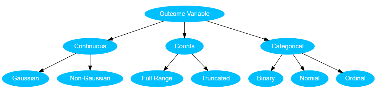
The decision tree methodology is used in random forests. For instance, when we chose to perform an analysis on an outcome variable or target our thinking might flow into this decision tree inspired from (Riggs and Lalonde 2017) in Figure 1
A decision tree is used to visually and analytically categorize data in which the expected values of competing alternatives are calculated (Everitt 2005). A decision tree (or root diagram) has a starting root and spreads into branches which in turn terminate in leaves. Each branch point is called a node and represents a decision based on an attribute (e.g., is an outcome variable continuous or counts or categorical as in Figure 1), each branch is the outcome of the decision, and each leaf represents a class label; i.e., a decision made after deciding all variable attributes such as whether a continuous variable is either Gaussian or non-Gaussian. The paths from the starting root to a leaf represent classification rules.
A decision tree consists of three types of nodes: Decision nodes, chance nodes, and terminus nodes or leaves. If decisions are to be made with no history and under incomplete knowledge, a decision tree is combined with a probability model as a best choice model or selection model algorithm. Another well-known use for decision trees is for calculating conditional probabilities.
Random Forest
A random forest may be thought of as a collection of many slightly different decision trees with branches split on database variable states or values (Liaw and Wiener 2002 [Online]). A decision tree, as described above, is a branching structure in which each node represents a decision based on variable state or value. The example described in this section is from (R. H. Hoover and Riggs 2018 [Online]). Each branch represents the outcome of a decision, and each terminus results in a class of either single layer ejecta (SLE), double layer (DLE), or multiple layer ejecta (MLE) after computing all other variable influences. The paths from root to leaf represent classification rules. Individual decision trees typically overfit the data and the bagging of multiple trees (ensembling) corrects each tree’s overfit by averaging over the classification rules.
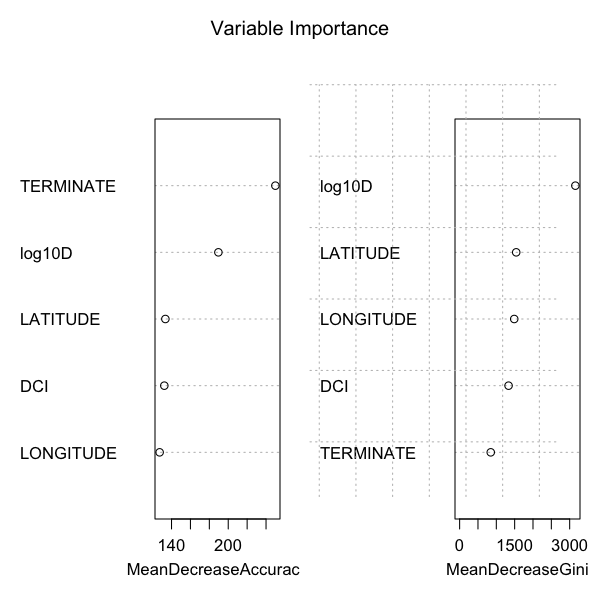
A random forest is a collection of many different decision trees constructed from, in this example, the Mars Thermal Inertia (TI) data set with the crater variables DIAMETER (\(\log_{10}(D)\), LATITUDE, LONGITUDE, dust cover index (DCI), layer terminate type, thermal inertia (\(\log_{10}\)(TI)), layer EDGE type, TESTYPE (measure of minima, medians, or maxima), and TIME (day or night observations); combinations of the levels and values of these variables result in leaves of crater layer classifications. Individual decision trees are bagged to correct each tree’s overfit by averaging. Each tree uses randomly shifted levels and values of the variables to form 500 unique combinations of nodes ultimately terminating in the layer levels. The key variables importance plot and table is given in Figure 2 and Table 1.
| Mean Gini | Variable Name |
|---|---|
| 3189.503 | log10D |
| 1543.426 | LATITUDE |
| 1486.232 | LONGITUDE |
| 1342.237 | DCI |
| 825.666 | TERMINATE |
| 644.107 | log10TI |
| 156.927 | EDGE |
| 87.634 | TESTYPE |
| 50.880 | TIME |
The normalized Gini coefficient (Gini 1997) measures the inequality among values of a probability distribution function (PDF). A coefficient of zero expresses perfect equality between two PDFs when all values are the same. A Gini coefficient of 1 (or 100%) expresses maximal inequality among values of the PDFs. Given the normalization of both the cumulative distributions of the tree values used to calculate the Gini coefficient, the measure is not overly sensitive to the specifics of the distributions but rather only on how values vary relative to the other values of a distribution.
A variable importance plot (Figure 2 shows the key five variables selected and plotted based on the unnormalized Gini goodness of fit statistics. These five variables, (\(\log_{10}\)) diameter, latitude, longitude, dust cover index (DCI), and terminate (pancake or rampart), have the greatest influence on crater layer classification via random forest ensemble method. A table with decreasing order of importance based on measures for model accuracy and node purity is given in Table 1. The Gini coefficient measures the inequality among values of a frequency distribution (mean from bagging) in which small values indicate a lack of node splitting differentiation and large values indicate maximal node splitting differentiation for the random forest variables.
A plot of the error rate in Figure 3 across decision trees suggests that after approximately 200 decision trees, there is not a significant reduction in error rate which suggests the choice of 500 trees for the crater data is adequate. Out-of-bag error is the mean prediction error on each training case, using only the trees that did not have that specific case in the bootstrap sample. 500 decision trees were selected for a forest using LAYERS as the response which falls within the lowest part of the error rate. (Liaw and Wiener 2002 [Online]) state that for each tree, the prediction accuracy on the out-of-bag portion of the data is recorded and the same after permuting each predictor variable. The difference between the two accuracies are then averaged over all trees, and normalized by the standard error.
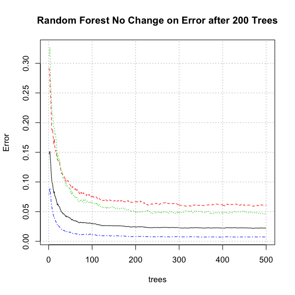
This analysis utilizes the random forest technique proposed by (Breiman 2001). His enhancement adds another layer of randomness to bagging each tree using a different bootstrap sample of the data; viz., random forests change how the classification or regression trees are constructed. Standard tree construction has each node partitioned using the best split among all variables. In a random forest, each node is split using the best among a subset of predictors randomly chosen at that node. The number of trees therefor needed to create the forest is lower than just the bagging of decision trees.
A confusion matrix or error matrix ( Table 2 ) based on the actual response variable and the predicted response value was constructed from the evaluation data set. Each row of the matrix represents the number in a predicted class (SLE, DLE, MLE) while each column represents the number in an actual class. The matrix is used to calculate if the system is confusing any one class with the others (i.e., a misclassification). The confusion matrix gives a classification accuracy of 0.982 with 95% CI (0.979, 0.984 (range 0 - 1, 1 being excellent) which is desirably significantly greater than the no information rate (NIR) of 0.695 as evidenced by the p-value of accuracy \(>\) NIR \(<<0.01\).
| Prediction | Reference | ||
|---|---|---|---|
| DLE | MLE | SLE | |
| DLE | 2447 | 35 | 37 |
| MLE | 17 | 1428 | 16 |
| SLE | 101 | 36 | 9191 |
Table 3 is the confusion matrix statistics for the three impact crater layer levels. Sensitivity is the true positive rate for which values near one show the evaluation data are correctly classified using the rules established by the training data set. Specificity is the true negative rate for which values near one indicate values of the evaluation data have few incorrect classifications based on the decision tree splittings of the training data. The positive predictive value (precision) and the negative predictive value each represent the accuracy of true positive and true negative classifications respectively. High values of these measures suggest correct leaf classifications. The detection rate is the overall probability of obtaining a correct classification. Detection prevalence is the proportion of the evaluation data classified as true out of all the evaluation data. Balanced accuracy is half the sum of sensitivity and selectivity with values near one suggesting correct classifications. Generally, the confusion matrix statistics show the evaluation data follow closely the classifications of the training data making the analysis adequate.
| Metric | DLE | MLE | SLE |
|---|---|---|---|
| Sensitivity | 0.954 | 0.953 | 0.994 |
| Specificity | 0.993 | 0.997 | 0.966 |
| Positive Predictive Value | 0.971 | 0.977 | 0.985 |
| Negative Predictive Value | 0.989 | 0.994 | 0.987 |
| Prevalence | 0.193 | 0.113 | 0.695 |
| Detection Rate | 0.184 | 0.107 | 0.691 |
| Detection Prevalence | 0.189 | 0.110 | 0.701 |
| Balanced Accuracy | 0.974 | 0.975 | 0.980 |
The Kappa statistic is a measure of concordance for categorical data that measures agreement relative to what would be expected by chance. The Kappa value is 0.961 with McNemar’s Test p-value of \(<< 0.01\) suggesting significant agreement. A value of 1 indicates perfect agreement and a value of zero indicates a lack of agreement. Kappa is an excellent performance measure when the classes are highly unbalanced as is the case for the TI data layer classes. the Kappa statistic supports the confusion matrix statistics of an adequate set of classification rules for the evaluation data.