2  Getting Started with R

In the first chapter, we introduce you to some base functionality within R and showcase how to perform some basic statistical tasks.

For starters, you can interface directly with the R Console and enter in basic calculations. Below we show a simple mathematical equation and how R appropriately returns the correct answer:

(2*3-1)^2 - 5 

[1] 20

Often we will want to save a value, to do this we use one of the assignment operators : <- , ->, or =, as you can see below the example below:

x <- 2*3 # left assign
2 -> y   # right assign 
z = 5    # equal assign
w <- (x-1)^y-z  

print(x)

[1] 6

print(y)

[1] 2

print(z)

[1] 5

print(w)

[1] 20

Above the print() function is used to output or display values to the console or output window. The print() function is often used to display the result of a computation or the value of a variable.

Alternatively, we also use the cat() function to print output to the console without the extra formatting that print() provides:

cat(w)

20

While you can use the -> assignment operator, for R you will most often see code formatted as:

thing_you_are_defining <- definition_of_the_thing

OR

thing_you_are_defining = definition_of_the_thing

In this text we will attempt to follow best practices in terms of formatting and syntax. We will try to reserve the <- assignment operation for defining new objects and = operator for setting parameters within a function. See https://style.tidyverse.org/index.html

2.1 Basic Data Types in R

R has 6 basic data types.

• numeric (real or decimal)
• integer
• character
• logical
• complex

The class function can let you know the data type:

class(3.14)

[1] "numeric"

# pi = R approximation for the mathematical constant pi
class(pi) 

[1] "numeric"

class(45)

[1] "numeric"

# add L if you want R to think of this as an integer
class(45L)

[1] "integer"

class("integer")

[1] "character"

# logical TRUE
class(TRUE) 

[1] "logical"

R can also handle complex numbers:

# the complex value of 2 + 3*sqrt(-1)
cx <- complex(length.out = 1, 
        real = 2, 
        imaginary = 3) 

cx

[1] 2+3i

class(cx)

[1] "complex"

R can also test if a statement is TRUE or FALSE, for example:¹

2 + 2 == 5

[1] FALSE

Note we use == to test logical statements as = is reserved for assignments or setting parameters within functions. There are several relational operators including:

Relational Operators

Relational operator	Meaning
<	less than
<=	less than or equal to
>	greater than
>=	greater than or equal to
==	equal to
!=	not equal to

Additionally, there are logical operators including:

Logical Operators

Logical Operator	Meaning
&	and
|	or
!	not

2.2 Summary of basic R Data Types

Summary of basic R Data Types

Example	Type
“male”, “Diabetes”	Character / String
3, 20.6, 100.222	Numeric
26L (add an ‘L’ to denote integer)	Integer
TRUE, FALSE	Logical
2+3i	Complex

2.3 Lists and Vectors

Lists and vectors are similar in R but a few differences separate them:

List	Vector
A list holds different data such as Numeric, Character, logical, etc.	Vector stores elements of the same type or converts implicitly.
list is a multidimensional object; elements in a list can have different lengths	The vector is one-dimensional; elements in a vector must have the same length
Lists are recursive	vector is not recursive
elements in a list can be named	elements in a list cannot be named

2.3.1 lists

In R the list is a function which allows one to create a collection of objects, which can be of different data types, such as numeric, character, or logical. The objects can also have different lengths.

my_list <- list(first_name = "John",
                last_name = "Doe",
                age = 30, 
                hobbies = c("reading", "swimming"))

my_list

$first_name
[1] "John"

$last_name
[1] "Doe"

$age
[1] 30

$hobbies
[1] "reading"  "swimming"

R provides many functions to examine features of lists, vectors and other objects, for example

• class() - what kind of object is it (high-level)?
• typeof() - what is the object’s data type (low-level)?
• length() - how long is it? What about two dimensional objects?
• attributes() - does it have any metadata?

class(my_list)

[1] "list"

length(my_list)

[1] 4

typeof(my_list)

[1] "list"

attributes(my_list)

$names
[1] "first_name" "last_name"  "age"        "hobbies"   

2.3.2 vectors

In contrast, a vector is a collection of elements of the same data type. In R, vectors can be numeric, character, or logical. We can make vectors within R by using the c() function, in the example below we make a few examples:

vector_of_ints <- c(2L,4L,6L,8L)

vector_of_strings <- c("Data", "Science", "is a", 'blast!')

vector_of_logicals <- c(TRUE, FALSE, TRUE, FALSE)

vector_of_mixed_type <- c(3.14, 1L, "cat", TRUE)

vector_of_numbers <- c(22/7, 18, 42, 65.2)

vector_of_sexes <- c("Male","Female","Female","Male")

class(vector_of_strings)

[1] "character"

length(vector_of_strings)

[1] 4

typeof(vector_of_strings)

[1] "character"

attributes(vector_of_strings)

NULL

class(vector_of_ints)

[1] "integer"

length(vector_of_ints)

[1] 4

typeof(vector_of_ints)

[1] "integer"

attributes(vector_of_ints)

NULL

class(vector_of_numbers)

[1] "numeric"

length(vector_of_numbers)

[1] 4

typeof(vector_of_numbers)

[1] "double"

attributes(vector_of_numbers)

NULL

class(vector_of_mixed_type)

[1] "character"

length(vector_of_mixed_type)

[1] 4

typeof(vector_of_mixed_type)

[1] "character"

attributes(vector_of_mixed_type)

NULL

Note above that the vector_of_mixed_type is coerced into a "charater" type to accommodate the variation of the different types of data within the vector definition.

2.3.2.1 Factors

Factors are often used to represent categorical data or data with a limited number of unique values into different levels. If we use the factor function on vector_of_sexes it returns back a factor object with the levels representing the unique values within the vector.

vector_of_sexes_factor <- factor(vector_of_sexes)
class(vector_of_sexes_factor)

[1] "factor"

vector_of_sexes_factor

[1] Male   Female Female Male  
Levels: Female Male

2.3.2.1.1 Levels and ordered levels

We can access the levels of a factor with the levels function:

levels(vector_of_sexes_factor)

[1] "Female" "Male"  

The order of the levels in a factor can be changed by applying the factor function again with new order of the levels:

vector_of_sexes_factor_relevel <- factor(vector_of_sexes, 
                                         levels = c("Male","Female"))
vector_of_sexes_factor_relevel

[1] Male   Female Female Male  
Levels: Male Female

We can also place an ordering on the factors with the ordered function :

vector_of_costs <- c('$200 - $300',
                     '$0 - $100',
                     '$300 - $400',
                     '$100 - $200')

costs_order <- c('$0 - $100',
                 '$100 - $200',
                 '$200 - $300',
                 '$300 - $400')

ordered_vector_of_costs <- ordered(vector_of_costs, 
                                   levels = costs_order)
ordered_vector_of_costs

[1] $200 - $300 $0 - $100   $300 - $400 $100 - $200
Levels: $0 - $100 < $100 - $200 < $200 - $300 < $300 - $400

class(ordered_vector_of_costs)

[1] "ordered" "factor" 

2.3.3 Accessing elements in a list or vector

We can access certain elements from within the indexing operator [[]] or [ ] with the name or index of the element:

my_list[1]

$first_name
[1] "John"

class(my_list[1])

[1] "list"

above we have a return of a new list that contains only the first element of my_list. This is useful when you want to extract a subset of the list and retain the information about the name and position of the element in the list.

Alternatively, if we want to return the element of the list as a separate object we can do so:

my_list[[1]]

[1] "John"

This is useful when you want to access the value of the first element directly, without retaining any information about its name or position in the list.

If the list is nested of contains multiple elements we can itterate the above steps:

my_list[[4]][2]

[1] "swimming"

Since our list named elements we can also access them with the element names:

my_list[["hobbies"]][2]

[1] "swimming"

Or, we can also utilize this notation as well:

my_list$hobbies[2]

[1] "swimming"

Similarly, we can access elements of a vector with the same [] operator, however, since vectors are of a single dimension, there is no ambiguity and a value will be returned:

vector_of_mixed_type[1]

[1] "3.14"

vector_of_mixed_type[2]

[1] "1"

vector_of_mixed_type[3]

[1] "cat"

vector_of_mixed_type[4]

[1] "TRUE"

list_of_vectors <- list(vector_of_ints,
                      vector_of_strings,
                      vector_of_logicals,
                      vector_of_mixed_type,
                      vector_of_numbers,
                      vector_of_sexes)

list_of_vectors

[[1]]
[1] 2 4 6 8

[[2]]
[1] "Data"    "Science" "is a"    "blast!" 

[[3]]
[1]  TRUE FALSE  TRUE FALSE

[[4]]
[1] "3.14" "1"    "cat"  "TRUE"

[[5]]
[1]  3.142857 18.000000 42.000000 65.200000

[[6]]
[1] "Male"   "Female" "Female" "Male"  

list_of_vectors[[2]][[4]]

[1] "blast!"

names(list_of_vectors) <- list('vector_of_ints',
                      'vector_of_strings',
                      'vector_of_logicals',
                      'vector_of_mixed_type',
                      'vector_of_numbers',
                      'vector_of_sexes')

list_of_vectors

$vector_of_ints
[1] 2 4 6 8

$vector_of_strings
[1] "Data"    "Science" "is a"    "blast!" 

$vector_of_logicals
[1]  TRUE FALSE  TRUE FALSE

$vector_of_mixed_type
[1] "3.14" "1"    "cat"  "TRUE"

$vector_of_numbers
[1]  3.142857 18.000000 42.000000 65.200000

$vector_of_sexes
[1] "Male"   "Female" "Female" "Male"  

list_of_vectors[['vector_of_strings']][[4]]

[1] "blast!"

2.4 Matrices

A matrix is a rectangular array or table of numbers, symbols, or expressions, arranged in rows and columns, which is used to represent a mathematical object or a property of such an object.

In R a matrix \(M\) is an \(n \times k\) array with \(n\) rows with \(k\) columns, we say the dimension of \(M\) is \(n \times k\). We can find the dimension of an R matrix with the dim function. We can use nrow to return the number of rows, similarly, ncol will return the number of columns.

M <- matrix(data = 1:20, 
            nrow = 4, 
            byrow = TRUE)

M

     [,1] [,2] [,3] [,4] [,5]
[1,]    1    2    3    4    5
[2,]    6    7    8    9   10
[3,]   11   12   13   14   15
[4,]   16   17   18   19   20

dim(M)

[1] 4 5

nrow(M)

[1] 4

ncol(M)

[1] 5

class(M)

[1] "matrix" "array" 

length(M)

[1] 20

typeof(M)

[1] "integer"

attributes(M)

$dim
[1] 4 5

2.4.1 Matrix Notation

We can use familiar matrix notation to select specific elements from the data frame:

M[row , column]

for example,

M[2,3]

[1] 8

We can use similar notation to select a row:

M[2,]

[1]  6  7  8  9 10

Or a column:

M[,3]

[1]  3  8 13 18

We can also subset on ranges of rows or columns:

M[2:4,3:5]

     [,1] [,2] [,3]
[1,]    8    9   10
[2,]   13   14   15
[3,]   18   19   20

We can also add on additional attributes to the matrix such as dimensional names:

colnames <- c("odd", "even", "prime", "composite")
 
rownames<- paste0("row",seq(1:5))

M <- matrix(data = c(1,  2,  2,  4, 
                     3,  4,  3,  6,
                     5,  6,  5,  8,
                     7,  8,  7,  9,
                     9, 10, 11, 10), 
            nrow = 5, 
            byrow = TRUE, 
            dimnames = list(rownames, colnames))
M

     odd even prime composite
row1   1    2     2         4
row2   3    4     3         6
row3   5    6     5         8
row4   7    8     7         9
row5   9   10    11        10

class(M)

[1] "matrix" "array" 

length(M)

[1] 20

typeof(M)

[1] "double"

attributes(M)

$dim
[1] 5 4

$dimnames
$dimnames[[1]]
[1] "row1" "row2" "row3" "row4" "row5"

$dimnames[[2]]
[1] "odd"       "even"      "prime"     "composite"

It is often important and helpful to have meaningful column names. This is useful for quickly understanding what variables you are viewing and logical for programming purposes. You can review the column names of a data frame with the colnames function.

It is also helpful to be able to pass in these column names to select a column rather than recall which column number the information is associated with:

M[,'prime']

row1 row2 row3 row4 row5 
   2    3    5    7   11 

or access a column:

M['row1',]

      odd      even     prime composite 
        1         2         2         4 

2.5 The Data Frame

A data frame is a two-dimensional array-like structure. Like a matrix, the dimension of a data frame is \(n \times k\) with \(n\) rows with \(k\) columns in which each column is a vector containing values of one type and each row contains one set of values from each column.

The primary difference between data frames and matrices is that data frames allow for columns to be of different datatypes. Additionally, there are many packages and methods which are specifically designed to deal with data frames or matrices. Often we may need to convert between a matrix or a data frame in order to properly utilize specific functions.

my_dataframe <- data.frame(vector_of_ints, 
                           vector_of_strings, 
                           vector_of_logicals, 
                           vector_of_mixed_type, 
                           vector_of_numbers,
                           vector_of_sexes_factor,
                           ordered_vector_of_costs)

my_dataframe

  vector_of_ints vector_of_strings vector_of_logicals vector_of_mixed_type
1              2              Data               TRUE                 3.14
2              4           Science              FALSE                    1
3              6              is a               TRUE                  cat
4              8            blast!              FALSE                 TRUE
  vector_of_numbers vector_of_sexes_factor ordered_vector_of_costs
1          3.142857                   Male             $200 - $300
2         18.000000                 Female               $0 - $100
3         42.000000                 Female             $300 - $400
4         65.200000                   Male             $100 - $200

class(my_dataframe)

[1] "data.frame"

length(my_dataframe)

[1] 7

typeof(my_dataframe)

[1] "list"

attributes(my_dataframe)

$names
[1] "vector_of_ints"          "vector_of_strings"      
[3] "vector_of_logicals"      "vector_of_mixed_type"   
[5] "vector_of_numbers"       "vector_of_sexes_factor" 
[7] "ordered_vector_of_costs"

$class
[1] "data.frame"

$row.names
[1] 1 2 3 4

We can see the first few rows of a data frame with the head function:

head(my_dataframe)

  vector_of_ints vector_of_strings vector_of_logicals vector_of_mixed_type
1              2              Data               TRUE                 3.14
2              4           Science              FALSE                    1
3              6              is a               TRUE                  cat
4              8            blast!              FALSE                 TRUE
  vector_of_numbers vector_of_sexes_factor ordered_vector_of_costs
1          3.142857                   Male             $200 - $300
2         18.000000                 Female               $0 - $100
3         42.000000                 Female             $300 - $400
4         65.200000                   Male             $100 - $200

As with matrices we can determine the dimension by using the dim function:

dim(my_dataframe)

[1] 4 7

so we can see that this data-frame has 4 rows and 7 columns. We can also get those values by using nrow and ncol:

nrow(my_dataframe)

[1] 4

ncol(my_dataframe)

[1] 7

As with matrices we can use either matrix notation to access certain rows or columns or ranges of values from the data frame:

my_dataframe[c(2,4) , c('vector_of_ints','vector_of_logicals','ordered_vector_of_costs') ]

  vector_of_ints vector_of_logicals ordered_vector_of_costs
2              4              FALSE               $0 - $100
4              8              FALSE             $100 - $200

In addition, to the matrix notion we covered above, we can access the column vector of a data frame with the $ notation.

my_dataframe$vector_of_strings

[1] "Data"    "Science" "is a"    "blast!" 

2.6 Structure

The R Structure function will compactly display the internal structure of an R object.

To see help page for a function use ? before the function name, for example try: ?str

For example, if we use str on my_dataframe it will show the user the number of observations, variables and data type of each list:

str(my_dataframe)

'data.frame':   4 obs. of  7 variables:
 $ vector_of_ints         : int  2 4 6 8
 $ vector_of_strings      : chr  "Data" "Science" "is a" "blast!"
 $ vector_of_logicals     : logi  TRUE FALSE TRUE FALSE
 $ vector_of_mixed_type   : chr  "3.14" "1" "cat" "TRUE"
 $ vector_of_numbers      : num  3.14 18 42 65.2
 $ vector_of_sexes_factor : Factor w/ 2 levels "Female","Male": 2 1 1 2
 $ ordered_vector_of_costs: Ord.factor w/ 4 levels "$0 - $100"<"$100 - $200"<..: 3 1 4 2

When we call str on ordered_vector_of_costs we see that it is a character vector of length 4 and are shown the values

str(ordered_vector_of_costs)

 Ord.factor w/ 4 levels "$0 - $100"<"$100 - $200"<..: 3 1 4 2

2.7 summary

The summary is a generic function used to produce summaries of the results of various model fitting functions.

See ?summary for more information.

In the case of a data frame the summary function will give summary level information on the data frame, for continuous variables it will display the minimum, first quartile, median, mean, third quartile and max; for categorical data counts of each of the classes

summary(my_dataframe)

 vector_of_ints vector_of_strings  vector_of_logicals vector_of_mixed_type
 Min.   :2.0    Length:4           Mode :logical      Length:4            
 1st Qu.:3.5    Class :character   FALSE:2            Class :character    
 Median :5.0    Mode  :character   TRUE :2            Mode  :character    
 Mean   :5.0                                                              
 3rd Qu.:6.5                                                              
 Max.   :8.0                                                              
 vector_of_numbers vector_of_sexes_factor ordered_vector_of_costs
 Min.   : 3.143    Female:2               $0 - $100  :1          
 1st Qu.:14.286    Male  :2               $100 - $200:1          
 Median :30.000                           $200 - $300:1          
 Mean   :32.086                           $300 - $400:1          
 3rd Qu.:47.800                                                  
 Max.   :65.200                                                  

We can also get these statistics by class, here we use the information in the data frame column vector_of_sexes

by(my_dataframe, 
   my_dataframe$vector_of_sexes, 
   summary)

my_dataframe$vector_of_sexes: Female
 vector_of_ints vector_of_strings  vector_of_logicals vector_of_mixed_type
 Min.   :4.0    Length:2           Mode :logical      Length:2            
 1st Qu.:4.5    Class :character   FALSE:1            Class :character    
 Median :5.0    Mode  :character   TRUE :1            Mode  :character    
 Mean   :5.0                                                              
 3rd Qu.:5.5                                                              
 Max.   :6.0                                                              
 vector_of_numbers vector_of_sexes_factor ordered_vector_of_costs
 Min.   :18        Female:2               $0 - $100  :1          
 1st Qu.:24        Male  :0               $100 - $200:0          
 Median :30                               $200 - $300:0          
 Mean   :30                               $300 - $400:1          
 3rd Qu.:36                                                      
 Max.   :42                                                      
------------------------------------------------------------ 
my_dataframe$vector_of_sexes: Male
 vector_of_ints vector_of_strings  vector_of_logicals vector_of_mixed_type
 Min.   :2.0    Length:2           Mode :logical      Length:2            
 1st Qu.:3.5    Class :character   FALSE:1            Class :character    
 Median :5.0    Mode  :character   TRUE :1            Mode  :character    
 Mean   :5.0                                                              
 3rd Qu.:6.5                                                              
 Max.   :8.0                                                              
 vector_of_numbers vector_of_sexes_factor ordered_vector_of_costs
 Min.   : 3.143    Female:0               $0 - $100  :0          
 1st Qu.:18.657    Male  :2               $100 - $200:1          
 Median :34.171                           $200 - $300:1          
 Mean   :34.171                           $300 - $400:0          
 3rd Qu.:49.686                                                  
 Max.   :65.200                                                  

2.8 Save and Read RDS files

You can save important data, variables, or models as R data files using the saveRDS function. This will save

saveRDS(my_dataframe , 'my_dataframe.RDS')

by default this saves to your working directory.

2.9 Where R we?

You can see your current working directory path by using getwd() :

getwd()

[1] "C:/Users/jkyle/Documents/GitHub/Jeff_R_Data_Wrangling/Part_1"

Note this might be different than what is returned by here::here()

here::here()

[1] "C:/Users/jkyle/Documents/GitHub/Jeff_R_Data_Wrangling"

You can alter the paths in a number of different ways.

In this example, we will want to save results to a sub-folder called y_data.

First, I will tell R to create a directory:

new_path <- file.path(getwd(),'y_data')

dir.create(new_path)

The above code creates a new directory called "y_data" in the current working directory of the R session.

• getwd() returns the current working directory of the R session, which is a character string representing the file path to the current directory.

• file.path() is a function that creates a file path from one or more path components. In this case, it combines the current working directory obtained from getwd() with the string "y_data".

The resulting file path is stored in the variable new_path. dir.create() is a function that creates a new directory with the specified name (in this case, "y_data") in the specified location (in this case, the current working directory). The function returns TRUE if the directory is successfully created, and FALSE otherwise.

The overall effect of the code is to create a new directory called "y_data" in the current working directory of the R session. If the directory already exists, dir.create() will not overwrite it and will return FALSE.

Now I can save y within this folder:

saveRDS(y, file.path(new_path,'y.RDS'))

Another useful package in this vain is the here package and the here function. The purpose of the here package is to simplify file path management in R projects. The here::here() function is used to generate a file path that is relative to the current project directory, rather than an absolute file path that is specific to the computer or operating system.

While in much of the older documentation for R you will see the use of setwd() to set the working directory, it is generally recommended to use the here package to set the working directory. This is because setwd() is not a robust way to set the working directory and can cause issues when sharing code with others.

The here package is much more robust, will work across different operating systems, and is generally a better practice in particular when working with others through GitHub or another version control system. Using here::here() to generate file paths that are relative to the project directory has several advantages over using absolute file paths. For example, it makes your code more portable, as you can move your project directory to a different location on your computer or to a different computer entirely, and the file paths will still be valid. It also makes it easier to collaborate with others on a project, as you don’t have to worry about differences in file paths between different computers or operating systems. We will install the here package through the majority of the text.

2.10 readRDS

You can load R data files by using readRDS :

z <- readRDS(file.path(new_path, 'y.RDS'))

y == z

[1] TRUE

2.11 Remove Items from your enviroment

WARNING once something is removed from your environment it is GONE! SAVE WHAT YOU NEED with saveRDS otherwise you will need to rerun portions of code.

You can remove items in your R environment by using the rm function.

rm(my_dataframe2)

Warning in rm(my_dataframe2): object 'my_dataframe2' not found

2.11.1 Remove all but a list

Let’s say that we want to remove everything except for my_dataframe and y, then we might do something like:

keep <- c('my_dataframe','new_path')

rm(list = setdiff(ls(), keep))

Above we are using multiple functions in conjunction with one-another:

1. We make a variable called keep to contain the items we wish to maintain
2. ls is returning a list of items within the environment
3. setdiff is taking the set-difference between ls which returns all the items within the environment and the items that we have specified within keep.

2.11.2 Delete Files / Folders

unlink deletes a file, we can use recursive = TRUE to delete directories:

unlink(new_path, recursive = TRUE)

2.12 Functions

A functionis an R object that takes in arguments or parameters and follows the collection of statements to provide the requested return.

2.12.1 Example R functions.

The R function set.seed is designed to assist with pseudo-random number generation.

The R function rnorm will produce a given number of randomly generated numbers from a normal distribution with a provided mean and standard-deviation. Below we define 4 distributions each of 1000 numbers:

• W will be drawn from a normal distribution with mean of 5 and standard deviation of 2.
• X, Y, and Z will be drawn from a normal distribution with mean of 0 and standard deviation of 1.
  • X and Z will be drawn with the same seed where as Y will be drawn with a different seed.

{
set.seed(12345)
X <- rnorm(1000, mean = 0, sd = 1)
}

{
set.seed(5)
Y <- rnorm(1000, mean = 0, sd = 1)
W <- rnorm(1000, mean = 5, sd = 2)
}


{
set.seed(12345)
Z <- rnorm(1000, mean = 0, sd = 1)
}

Here are the first 5 from each of the distributions:

cat("W \n")

W 

W[1:5]

[1] 2.089891 7.489126 4.136106 5.013739 5.249102

cat("X \n")

X 

X[1:5]

[1]  0.5855288  0.7094660 -0.1093033 -0.4534972  0.6058875

cat("Y \n")

Y 

Y[1:5]

[1] -0.84085548  1.38435934 -1.25549186  0.07014277  1.71144087

cat("Z \n")

Z 

Z[1:5]

[1]  0.5855288  0.7094660 -0.1093033 -0.4534972  0.6058875

Note that X and Z will be exactly the same sets since we used the same seed to generate the two sets of numbers whereas Y will be different, even though we used the same parameters, for example

X[546] == Z[546]

[1] TRUE

X[546] == Y[546]

[1] FALSE

Even though X and Y are not the same, they are sampled from the same distribution therefore the p-value on the t-test should be well above .05:

t.test(X,Y)

    Welch Two Sample t-test

data:  X and Y
t = 0.6405, df = 1997.7, p-value = 0.5219
alternative hypothesis: true difference in means is not equal to 0
95 percent confidence interval:
 -0.05938059  0.11697799
sample estimates:
 mean of x  mean of y 
0.04619816 0.01739946 

Comparatively, X and W were not sampled from the same distribution, therefore the p-value should be closer to 0:

t.test(X,W)

    Welch Two Sample t-test

data:  X and W
t = -72.569, df = 1474.2, p-value < 2.2e-16
alternative hypothesis: true difference in means is not equal to 0
95 percent confidence interval:
 -5.237795 -4.962086
sample estimates:
 mean of x  mean of y 
0.04619816 5.14613865 

We will review the t-test in greater detail in Section 6.1.

We can see the difference between the distributions by using the hist function in Figure 2.1:

hist(X, 
     col=rgb(1,0,0,0.5), # red
     main="Overlapping Histogram") 
hist(Y, 
     col=rgb(0,1,0,0.5), # green 
     add=T) 
hist(W, 
     col=rgb(0,0,1,0.5), # blue 
     add=T)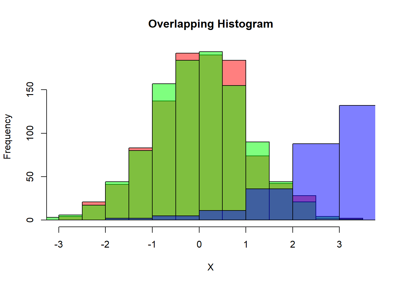  

Figure 2.1: Overlapping Histogram of X, Y, & W

We will cover graphing with R in greater detail in Chapter 5.

2.12.1.1 if-else

The if() function in R is a conditional statement that allows you to execute different code based on whether a specified condition is TRUE or FALSE.

The basic syntax for if function is as follows:

if (condition) {
  # code to execute if condition is TRUE
}

Above the condition is a logical expression that evaluates to either TRUE or FALSE. If the condition is TRUE, the code inside the curly braces {} will be executed. If the condition is FALSE, the code inside the curly braces {} will be skipped.

Optionally, you can add an else if or else clauses to execute different code if the initial condition is FALSE. The general syntax is as follows:

if ( condition1 ) {
  # code to execute if condition1 is TRUE
  } else if ( condition2 ) {
    # code to execute if condition2 is TRUE
    } else if ( condition3 ) {
      # code to execute if condition3 is TRUE
      } else {
        # code to execute if neither condition1, condition2, or condition3 is true.  
      }

x <- 56
y <- 56

if(x > y) {
  print("x is greater")
  } else if(x < y) {
    print("y is greater")
    } else {
      print("x and y are equal")
      }

[1] "x and y are equal"

2.12.1.2 for loop

The for() loop in R is a control structure that allows you to execute a block of code repeatedly for a specified number of times or for each element in a sequence.

Here’s the basic syntax of the for() loop:

for (variable in sequence) {
  # code to execute
}

The for loop below will iterate over all of the values in the lists in X and Z and check to see if they are not equal:

for(i in 1:1000){
  if(X[i] != Z[i]){
    print(paste0("i is ",i," and X[i] = ", X[i]," while Z[i] = ",Z[i]))
  }
}

2.12.1.3 while loop

while (test_expression) {
  statement
  }

Listing 2.1: Factorial calculation using a while loop

product <- 1

n <- 5

while (n >= 1){
  product <- product*n
  n <- n-1
}

1. Initialize the product variable to 1.
2. Initialize the n variable to 5.
3. The while loop will continue to execute as long as the value of n is greater than or equal to 1.
4. Multiply the product by n and assign the result back to product.
5. Decrease the value of n by 1.

Notice that this changes the value of n and product:

n

[1] 0

product

[1] 120

2.12.2 User defined functions

Thus far, all of the functions we have discussed come equipped with R, however, we are able to define our own functions with the function keyword. One advantage of defining your own functions is that you can reuse the code in the function as many times as you like. Additionally, the computation of the function is encapsulated within the function. This means that the variables defined within the function are not accessible outside of the function. This is known as the scope of the variable.

2.12.2.1 Factorial Example

For example, consider Listing 2.1 and compare it with a user-defined function Listing 2.2:

Listing 2.2: Factorial calculation using a user-defined function

product <- 1
n <- 5

my_factorial <- function(n){
  product <- 1
  while (n >= 1){
    product <- product*n
    n <- n-1
  }
  return(product)
}

my_factorial(5)

n
product

my_factorial(n)

[1] 120
[1] 5
[1] 1
[1] 120

1. Initialize the product variable to 1, note this is outside of the function definition.
2. Initialize the n variable to 5, note this is outside of the function definition.
3. We define a function called my_factorial() that takes a single argument n.
4. Initialize the product variable to 1, note this is inside of the function definition.
5. The while loop will continue to execute as long as the value of n is greater than or equal to 1.
6. Multiply the product by n and assign the result back to product.
7. Decrease the value of n by 1.
8. The return() function is used to return the value of product to the user.
9. The function my_factorial() is called with the argument 5.
10. The value of n is still 5.
11. The value of product is still 1.
12. The function my_factorial() is called with the argument n.

2.12.2.2 Quadratic Formula Example

Many of you may recall the quadratic formula from algebra; given a general quadratic equation of the form:

\[ax^2 + bx + c = 0 \]

with \(a\), \(b\), and \(c\) representing constants with \(a \neq 0\) then

\[x = -b \pm \frac{\sqrt{b^2 - 4ac}}{2a}\]

are the two solutions or roots of the quadratic equation.

We can program an R function that takes in as inputs the coefficients from a quadratic equation and returns the solutions for \(x\):

1quadratic_forumla <- function(a,b,c, quadratic = TRUE){
2  if(!is.logical(quadratic)){stop("quadratic must be a logical value")}
3  if(!(is.numeric(a) & is.numeric(b) & is.numeric(c))){
    stop("a, b, and c must be numeric")
  }
4  if(a == 0 & quadratic == TRUE){stop("a must not be 0.")}
5  if(a == 0 & quadratic == FALSE){
    print(paste0("Not a quadratic equation, the real solution is: x = ", -c/b))
    return(-c/b)
    }
  
6  D <- b^2 - 4*a*c
  
7  if(D >= 0){
    x_1 <- (-b + sqrt(D))/(2*a)
    x_2 <- (-b - sqrt(D))/(2*a)
    
8    if(D == 0){
      print(paste0("For ",a,"x^2 + ",b,"x"," + ",c," = 0; the real solution is: ", "x = ", x_1))
      return(x_1)
    }
    
9    print(paste0("For ",a,"x^2 + ",b,"x"," + ",c," = 0; the real solutions are: ", "x_1 = ", x_1, " and ", "x_2 = ", x_2))

    return(c(x_1, x_2))
    }
    
  
10  if(D < 0){
    Dc <- complex(1,D,0)
    
    x_1 <- (-b + sqrt(Dc))/(2*a)
    x_2 <- (-b - sqrt(Dc))/(2*a)
    
    print(paste0("For ",a,"x^2 + ",b,"x"," + ",c," = 0; the complex solutions are: ", "x_1 = ", x_1, " and ", "x_2 = ", x_2))

    return(c(x_1, x_2))
    }
}

1

Define a function called quadratic_formula() that takes three arguments a, b, and c. The quadratic argument is a logical value that defaults to TRUE.

2

Check if the quadratic argument is a logical value, if not stop the function and return an error message.

3

Check if a, b, and c are numeric, if not stop the function and return an error message.

4

Check if a is equal to 0, if so stop the function and return an error message.

5

Another option would be to assume the user is working with a linear equation and return the real solution.

6

Calculate the discriminant \(D = b^2 - 4ac\).

7

If the discriminant is greater than or equal to 0, calculate the two real roots of the quadratic equation.

8

If the discriminant is equal to 0, print the real solution and return the value of x_1.

9

If the discriminant is greater than 0, print the two real solutions and return a vector of the two solutions.

10

If the discriminant is less than 0, calculate the two complex roots of the quadratic equation and return a vector of the two solutions.

Important 2.1: Test Functions

It is important to test your functions with a variety of inputs to ensure they are working as expected.

2.12.2.3 Quadratic Formula Examples and Tests

We can explicitly name the parameters:

quadratic_forumla(a=1, b=5, c=6)

[1] "For 1x^2 + 5x + 6 = 0; the real solutions are: x_1 = -2 and x_2 = -3"

[1] -2 -3

When we explicitly name the parameters and we can pass them in any order:

quadratic_forumla(c=3, a=2, b=5)

[1] "For 2x^2 + 5x + 3 = 0; the real solutions are: x_1 = -1 and x_2 = -1.5"

[1] -1.0 -1.5

Or we can implicitly pass the parameters, however, here the function will assume they are being passed in which they are defined within the function:

1quadratic_forumla(1, 0, 4)

1

Assumes a = 1, b = 0, and c = 4 and quadratic defaults to TRUE.

[1] "For 1x^2 + 0x + 4 = 0; the complex solutions are: x_1 = 0+2i and x_2 = 0-2i"
[1] 0+2i 0-2i

Note that in the tests above we did not specify the quadratic argument, so it will default to TRUE, we can also test the function with quadratic = FALSE:

quadratic_forumla(0, 3, -15, quadratic = FALSE)

[1] "Not a quadratic equation, the real solution is: x = 5"

[1] 5

and as expected when we do not have a quadratic equation and leave quadratic = FALSE the function will return an error to the user.

quadratic_forumla(0, 3, -15)

Error in quadratic_forumla(0, 3, -15): a must not be 0.

This leads to an important point, when working with functions it is important to review the warnings and errors that are returned. This can help you identify issues with the function and make necessary corrections. Often times, the author of the function or package has included these messages to help you understand what went wrong.

Important 2.2: Review Warnings and Errors

When working with functions, it is important to review the warnings and errors that are returned. This can help you identify issues with code to ensure that you are getting the expected results.

We will cover additional examples of creating and utilizing user defined functions throughout the text.

2.13 Libraries & Packages

You may want to use newer or more specialized packages or libraries to read in or handle data. First we will need to make sure the library is installed with install.packages('package_name') then we can load the library with library('package_name') , and we will have access to all of the functionality withing the package.

Additionally, we can access a function from a library without loading the entire library, this can be done by using a command such as package::function, for instance, readr::read_csv tells R to look in the readr package for the function read_csv. This can be useful in programming functions and packages as well as if multiple packages contain functions with the same name.

2.13.1 installed packages

To see which packages are installed on your machine you can use the installed.packages() function.

The following function will check if a list of packages are already installed, if not then it will install them:

install_if_not <- function( list.of.packages ) {

  new.packages <- list.of.packages[!(list.of.packages 
                                     %in% 
                                    installed.packages()[,"Package"])]
  
  if(length(new.packages)) { 
    install.packages(new.packages, 
                     repos = "http://cran.us.r-project.org") }
  else { 
    print(paste0("the package '",
                 list.of.packages ,
                 "' is already installed")) }
}

You can use the function like this:

install_if_not(c("tidyverse"))

[1] "the package 'tidyverse' is already installed"

some additional information on the installed packages including the version can be found:

tibble::as_tibble(installed.packages()) |>
  dplyr::glimpse()

Rows: 369
Columns: 16
$ Package               <chr> "abind", "Amelia", "AMR", "archive", "arsenal", …
$ LibPath               <chr> "C:/Users/jkyle/Documents/GitHub/Jeff_R_Data_Wra…
$ Version               <chr> "1.4-5", "1.8.2", "2.1.1", "1.1.8", "3.6.3", "1.…
$ Priority              <chr> NA, NA, NA, NA, NA, NA, NA, NA, NA, NA, NA, NA, …
$ Depends               <chr> "R (>= 1.5.0)", "R (>= 3.0.2), Rcpp (>= 0.11)", …
$ Imports               <chr> "methods, utils", "foreign, utils, grDevices, gr…
$ LinkingTo             <chr> NA, "Rcpp (>= 0.11), RcppArmadillo", NA, "cli", …
$ Suggests              <chr> NA, "tcltk, broom, rmarkdown, knitr", "cli, curl…
$ Enhances              <chr> NA, NA, "cleaner, ggplot2, janitor, skimr, tibbl…
$ License               <chr> "LGPL (>= 2)", "GPL (>= 2)", "GPL-2 | file LICEN…
$ License_is_FOSS       <chr> NA, NA, NA, NA, NA, NA, NA, NA, NA, NA, NA, NA, …
$ License_restricts_use <chr> NA, NA, NA, NA, NA, NA, NA, NA, NA, NA, NA, NA, …
$ OS_type               <chr> NA, NA, NA, NA, NA, NA, NA, NA, NA, NA, NA, NA, …
$ MD5sum                <chr> NA, NA, NA, NA, NA, NA, NA, NA, NA, NA, NA, NA, …
$ NeedsCompilation      <chr> "no", "yes", "no", "yes", "no", "no", "yes", "no…
$ Built                 <chr> "4.4.0", "4.4.0", "4.4.0", "4.4.0", "4.4.0", "4.…

2.14 Using Packages

Just because we installed the package does not mean that R will be able to access it. We need to load the packages we wish to use with the library command. To check which packages are loaded you can use:

(.packages())

[1] "stats"     "graphics"  "grDevices" "datasets"  "utils"     "methods"  
[7] "base"     

Make sure that the tidyverse and dplyr packages are installed. You can run install.packages(c('tidyverse','dplyr')) to install both.

For this example we will load data we previously saved:

my_dataframe <- readRDS('my_dataframe.RDS' )

We can use the head command to remind ourselves of the first few rows:

head(my_dataframe)

  vector_of_ints vector_of_strings vector_of_logicals vector_of_mixed_type
1              2              Data               TRUE                 3.14
2              4           Science              FALSE                    1
3              6              is a               TRUE                  cat
4              8            blast!              FALSE                 TRUE
  vector_of_numbers vector_of_sexes_factor ordered_vector_of_costs
1          3.142857                   Male             $200 - $300
2         18.000000                 Female               $0 - $100
3         42.000000                 Female             $300 - $400
4         65.200000                   Male             $100 - $200

We make sections of code accessible to installed packages by using library command:

loaded_package_before <- (.packages())

# everthing below here can call functions in dplyr package
library('dplyr')

Attaching package: 'dplyr'

The following objects are masked from 'package:stats':

    filter, lag

The following objects are masked from 'package:base':

    intersect, setdiff, setequal, union

# glimpse is a function within the dplyr library, similar to head
glimpse(my_dataframe)

Rows: 4
Columns: 7
$ vector_of_ints          <int> 2, 4, 6, 8
$ vector_of_strings       <chr> "Data", "Science", "is a", "blast!"
$ vector_of_logicals      <lgl> TRUE, FALSE, TRUE, FALSE
$ vector_of_mixed_type    <chr> "3.14", "1", "cat", "TRUE"
$ vector_of_numbers       <dbl> 3.142857, 18.000000, 42.000000, 65.200000
$ vector_of_sexes_factor  <fct> Male, Female, Female, Male
$ ordered_vector_of_costs <ord> $200 - $300, $0 - $100, $300 - $400, $100 - $2…

(.packages())

[1] "dplyr"     "stats"     "graphics"  "grDevices" "datasets"  "utils"    
[7] "methods"   "base"     

loaded_package_after <- (.packages())

# setdiff will return the differences between the two sets
setdiff(loaded_package_after, loaded_package_before)

[1] "dplyr"

To remove a package from the R session we use the detach command:

detach(package:dplyr)
#the dplyr package has now been detached. calls to functions may have errors

packages_cur <- (.packages())

setdiff(loaded_package_after,packages_cur)

[1] "dplyr"

Additionally, we can access a function from a library without loading the entire library, this can be done by using a command such as package::function. This notation is needed in any instance where two or more loaded packages have at least one function with the same name. This notation is also useful in development of functions and packages.

For instance, the glimpse function from the dplyr package can also be accessed by using the following command

# glimpse the data
dplyr::glimpse(my_dataframe)

Rows: 4
Columns: 7
$ vector_of_ints          <int> 2, 4, 6, 8
$ vector_of_strings       <chr> "Data", "Science", "is a", "blast!"
$ vector_of_logicals      <lgl> TRUE, FALSE, TRUE, FALSE
$ vector_of_mixed_type    <chr> "3.14", "1", "cat", "TRUE"
$ vector_of_numbers       <dbl> 3.142857, 18.000000, 42.000000, 65.200000
$ vector_of_sexes_factor  <fct> Male, Female, Female, Male
$ ordered_vector_of_costs <ord> $200 - $300, $0 - $100, $300 - $400, $100 - $2…

And just notice that without the library loaded or the dplyr:: in front we can error:

# error
glimpse(my_dataframe)

Error in glimpse(my_dataframe): could not find function "glimpse"

After first detaching a package with detach(package.name.here) we can check for an update from the console with install.packages(c("package.name.here"))

install.packages(c('dplyr'), repos = "http://cran.us.r-project.org")

If a package has a lock you can override the lock with

install.packages(c('dplyr'), 
                 repos = "http://cran.us.r-project.org",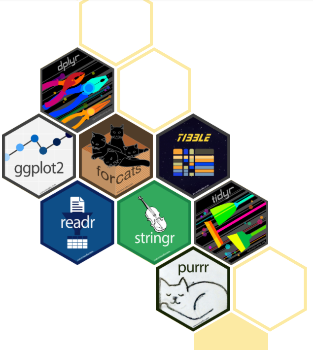 
                 INSTALL_opts = '--no-lock')

2.15 Welcome to the tidyverse

The tidyverse (Wickham et al. 2019) is a meta-package, a collection of R packages that have been grouped together in order to make “data wrangling” more efficient:

library('tidyverse')

── Attaching core tidyverse packages ──────────────────────── tidyverse 2.0.0 ──
✔ dplyr     1.1.4     ✔ readr     2.1.5
✔ forcats   1.0.0     ✔ stringr   1.5.1
✔ ggplot2   3.5.1     ✔ tibble    3.2.1
✔ lubridate 1.9.3     ✔ tidyr     1.3.1
✔ purrr     1.0.2     
── Conflicts ────────────────────────────────────────── tidyverse_conflicts() ──
✖ dplyr::filter() masks stats::filter()
✖ dplyr::lag()    masks stats::lag()
ℹ Use the conflicted package (<http://conflicted.r-lib.org/>) to force all conflicts to become errors

• tibble is an more modern R version of a data frame

• readr read in data-files such as CSV as tibbles or data-frames, write data-frames or tibbles to CSV or supported data-file type.

• dplyr is a popular package to manage many common data manipulation tasks and data summaries

• dbplyr database back-end for dplyr

• tidyr reshape your data but keep it ‘tidy’

• stringr functions to support working with text strings.

• purrr functional programming for R

• ggplot2 is an interface for R to create numerous types of graphics of data

• forcats tools for dealing with categorical data

• broom make outputs tidy

• lubridate working with dates

• readxl the readxl package contains the read_excel to read in .xls or .xlsx files

https://www.tidyverse.org/

2.15.1 and friends

Since the initial release of the tidyverse many other packages have been added to the tidyverse family. Some of these include:

• rmarkdown produce outputs such as HTML, PDF, Docs, PowerPoint.
• knitr extend the functionality of rmarkdown.
• quarto a new package for creating documents with R Markdown. See also https://quarto.org/.
• shiny Shiny is an R package that makes it easy to build interactive web apps straight from R.
• flexdashboard build dashboards with R
• furrr parallel mapping
• yardstick for model evaluation metrics

tidyverse_friends <- c('rmarkdown','knitr','quarto','shiny','flexdashboard','furrr','yardstick')

install.packages(tidyverse_friends)

2.15.2 pipe opperator

The pipe operator %>% \index{%>%} originates from the magrittr package. The pipe takes the information on the left and passes it to the information on the right:

Important 2.3: Pipe Operator

f(x) is the same as x %>% f()

Notice how x gets piped into a function f

glimpse(my_dataframe)

Rows: 4
Columns: 7
$ vector_of_ints          <int> 2, 4, 6, 8
$ vector_of_strings       <chr> "Data", "Science", "is a", "blast!"
$ vector_of_logicals      <lgl> TRUE, FALSE, TRUE, FALSE
$ vector_of_mixed_type    <chr> "3.14", "1", "cat", "TRUE"
$ vector_of_numbers       <dbl> 3.142857, 18.000000, 42.000000, 65.200000
$ vector_of_sexes_factor  <fct> Male, Female, Female, Male
$ ordered_vector_of_costs <ord> $200 - $300, $0 - $100, $300 - $400, $100 - $2…

is the same as

my_dataframe %>%
 glimpse()

Rows: 4
Columns: 7
$ vector_of_ints          <int> 2, 4, 6, 8
$ vector_of_strings       <chr> "Data", "Science", "is a", "blast!"
$ vector_of_logicals      <lgl> TRUE, FALSE, TRUE, FALSE
$ vector_of_mixed_type    <chr> "3.14", "1", "cat", "TRUE"
$ vector_of_numbers       <dbl> 3.142857, 18.000000, 42.000000, 65.200000
$ vector_of_sexes_factor  <fct> Male, Female, Female, Male
$ ordered_vector_of_costs <ord> $200 - $300, $0 - $100, $300 - $400, $100 - $2…

Note that this pipe operation has become so popular in R that version 4.1.0 and above now comes equipped with a pipe operator |> of it’s own without the use of the magrittr pipe operator:

1:10 |> mean()

[1] 5.5

Throughout the majority of this text we will be using the tidyverse packages and as such we will often defer to the magrittr pipe operator %>%.

Important 2.4: Pipe Operator Differences

Note there are subtle yet, substantial differences in how %>% and |> handle the passing of arguments to functions and performance. For more information see Chapter 15

2.15.3 Other Packages

Other packages we that will will make use of throughout the course of the text:

• devtools develop R packages

  • Note that devtools on Windows also requires Rtools https://cran.r-project.org/bin/windows/Rtools/

• arsenal compare data frames ; create summary tables

• skimr automate Exploratory Data Analysis

• DataExplorer automate Exploratory Data Analysis

• rsq computes Adjusted R² for various model types

• RSQLite R package for interfacing with SQLite database

• plotly interactive HTML plots

• DT contains datatable function for interactive HTML datatable

• GGally contains ggcorr for correlation plots and ggpairs for other data-plots

• corrr correlation matrix as a data-frame

• corrplot packge to assist with visulaization of correlations

• AMR Principal Component Plots

• randomForest fit a Random Forest model

• caret (Classification And Regression Training) is a set of functions that attempt to streamline the process for creating predictive models. Note that the caret package is no longer receiving support and users are encouraged to utilize the tidymodels framework.

• tidymodels is a collection of packages for modeling and machine learning using the tidyverse. We recommend (Kuhn and Silge 2022) for a detailed introduction to the tidymodels package.

• usethis usethis is a workflow package; it automates repetitive tasks that arise during project setup and development, both for R packages and non-package projects.

• testthat testthat is a package designed to assist with unit testing functions within packages.

• pkgdown pkgdown is designed to make it quick and easy to build a website for your package.

• here simplify file path management in R projects.

• renv records the version of R + R packages being used in a project, and provides tools for reinstalling the declared versions of those packages in a project.

other_packages <- c('devtools', 'rsq', 'arsenal', 'skimr',
                    'DataExplorer', 'RSQLite', 'dbplyr',
                    'plotly', 'DT', 'GGally', 
                    'corrr','AMR', 'caret', 
                    'randomForest','shiny','usethis',
                    'testthat', 'pkgdown', 'here',
                    'renv')

install.packages(other_packages)

2.16 Package Versions

We already mentioned that install.packages will update the package from CRAN. We can also use the function from the devtools package to install the most-up-to-date package from github, for example:

devtools::install_github("tidyverse/tidyverse")

Here are the versions installed on this system, compare with your own:

my_tidyverse_pack <- tidyverse::tidyverse_packages()

installed.packages() |>
  dplyr::as_tibble() |>
  dplyr::select(Package, Version, Depends) |> 
  dplyr::filter(Package %in% 
           c(my_tidyverse_pack, 
             tidyverse_friends , 
             other_packages)) |>
  knitr::kable()

Package	Version
base	4.4.1
DBI	1.2.3
dbplyr	2.5.0
dplyr	1.1.4
here	1.0.1
knitr	1.47
microbenchmark	1.4.10
rmarkdown	2.27
RSQLite	2.3.7
tibble	3.2.1
tidyr	1.3.1
tidyverse	2.0.0

devtools::install_version("dplyr", version = "1.0.10")

Another good option to ensure version control is to build a package or use the R package renv.

2.17 Details on this machine’s version of R

Below we provide some code which works as follows:

• The Sys.info() function is called, which returns a named character vector containing information about the current operating system.

• The tibble::enframe() function is called to convert the named character vector into a tibble (a type of data frame) with two columns: name and value. The name column contains the names of the elements in the original vector, and the value column contains the values of those elements.

• The filter() function is called to select only the rows of the tibble where the name column matches one of the four operating system properties of interest: sysname, release, version, and machine.

• Finally, the knitr::kable() function is called to format the resulting tibble as a table that can be printed or displayed in a document.

Sys.info() |>
  tibble::enframe() |>
  dplyr::filter(name %in% c('sysname','release','version','machine')) |>
  knitr::kable()

name	value
sysname	Windows
release	10 x64
version	build 22631
machine	x86-64

Below we use the R.Version() function, which returns a list containing information about the current version of R. Then the tibble::as_tibble() is used to convert the list output of R.Version() into a tibble. Next, the tidyr::pivot_longer() function is called to pivot the resulting tibble into a longer format, where each row represents a single element of the list output of R.Version(). The everything() argument tells pivot_longer() to pivot all columns of the tibble. And finally, the knitr::kable() function is called to format the resulting tibble as a table that can be printed or displayed in a document.

R.Version() |>
  tibble::as_tibble() |>
  tidyr::pivot_longer(everything()) |>
  knitr::kable()

name	value
platform	x86_64-w64-mingw32
arch	x86_64
os	mingw32
crt	ucrt
system	x86_64, mingw32
status
major	4
minor	4.1
year	2024
month	06
day	14
svn rev	86737
language	R
version.string	R version 4.4.1 (2024-06-14 ucrt)
nickname	Race for Your Life

2.17.1 sessionInfo

The sessionInfo command displays information about the current version of R, the operating system and the packages that are currently loaded or attached:

sessionInfo()

R version 4.4.1 (2024-06-14 ucrt)
Platform: x86_64-w64-mingw32/x64
Running under: Windows 11 x64 (build 22631)

Matrix products: default


locale:
[1] LC_COLLATE=English_United States.utf8 
[2] LC_CTYPE=English_United States.utf8   
[3] LC_MONETARY=English_United States.utf8
[4] LC_NUMERIC=C                          
[5] LC_TIME=English_United States.utf8    

time zone: America/New_York
tzcode source: internal

attached base packages:
[1] stats     graphics  grDevices datasets  utils     methods   base     

other attached packages:
 [1] lubridate_1.9.3 forcats_1.0.0   stringr_1.5.1   dplyr_1.1.4    
 [5] purrr_1.0.2     readr_2.1.5     tidyr_1.3.1     tibble_3.2.1   
 [9] ggplot2_3.5.1   tidyverse_2.0.0

loaded via a namespace (and not attached):
 [1] grateful_0.2.4    gtable_0.3.5      jsonlite_1.8.8    compiler_4.4.1   
 [5] renv_1.0.7        tidyselect_1.2.1  scales_1.3.0      yaml_2.3.8       
 [9] fastmap_1.2.0     here_1.0.1        R6_2.5.1          generics_0.1.3   
[13] knitr_1.47        htmlwidgets_1.6.4 munsell_0.5.1     rprojroot_2.0.4  
[17] pillar_1.9.0      tzdb_0.4.0        rlang_1.1.4       utf8_1.2.4       
[21] stringi_1.8.4     xfun_0.45         timechange_0.3.0  cli_3.6.3        
[25] withr_3.0.0       magrittr_2.0.3    digest_0.6.36     grid_4.4.1       
[29] rstudioapi_0.16.0 hms_1.1.3         lifecycle_1.0.4   vctrs_0.6.5      
[33] evaluate_0.24.0   glue_1.7.0        fansi_1.0.6       colorspace_2.1-0 
[37] rmarkdown_2.27    tools_4.4.1       pkgconfig_2.0.3   htmltools_0.5.8.1

Kuhn, Max, and Julia Silge. 2022. Tidy Modeling with R. Sebastopol, CA: O’Reilly Media.

Wickham, Hadley, Mara Averick, Jennifer Bryan, Winston Chang, Lucy McGowan, Romain François, Garrett Grolemund, et al. 2019. “Welcome to the Tidyverse.” J. Open Source Softw. 4 (43): 1686.

---

1. According to an old joke and as a homage to the novel 1984 by George Orwell, this may be true for for extremely large values of 2.