3 The `tidyverse`

3.1 Connect to SQLite database

Our first step will be to connect to the NHANES database using the DBI package. Please ensure that you have the here, DBI, tidyverse, RSQLite and dbplyr packages installed.

If not, you can install it using the following commands: install.packages('here'), install.packages('tidyverse'), install.packages('DBI'), install.packages('dbplyr'), install.packages(RSQLite) . If you saved the database in a different location, please update the path in the here function to match the path to where you have stored the file.

Code

library("DBI")
library("tidyverse")
library("dbplyr")

NHANES_DB <- DBI::dbConnect(
  RSQLite::SQLite(), # SQLite driver
  here::here("DATA/sql_db/NHANES.sqlite") # Path to the NHANES database,
  # user = "jka011", # not needed in this case 
  # password = rstudioapi::askForPassword()  
  )

Above:

DBI::dbConnect(): This is a function from the DBI package that establishes a connection to a database.
RSQLite::SQLite(): This is a function from the RSQLite package that specifies the SQLite driver, which is needed to connect to an SQLite database.
here::here("DATA/sql_db/NHANES.sqlite"): We use here::here to construct a file path.
while user and password are not needed in this case they will often be required when connecting to a database. If the database required a username for connection, you would uncomment this line and replace user with the required username.
Notice above we have used rstudioapi::askForPassword() to prompt the user for a password. We recommend that you do not hard code passwords in your code.
- Use the keyring https://keyring.r-lib.org/ or similar package to store passwords securely.
- You can also store your GitHub token with keyring or with the credentials https://docs.ropensci.org/credentials/ package.
- One final option is to use the usethis::edit_r_environ() function to add an environmental variable store your password in the .Renviron file. Note this is not as secure as the other options.
  1. The .Renviron file stores environment variables in plain text. This means that anyone who can access this file can see the passwords or other sensitive information it contains.
  2. The security of the .Renviron file depends on the file system permissions. If the file permissions are not set correctly or you are working on a shared machine unauthorized users might be able to read the file.
  3. If you’re using a version control system like Git, you need to be careful not to accidentally commit the .Renviron file, as this would expose your passwords to anyone who has access to your repository.
  4. The .Renviron file does not support encryption. This means that the passwords are not stored in a secure manner

Important 3.1: DO NOT HARD CODE PASSWORDS

It is important to never hard code passwords in your code. This is a security risk. Instead, consider the following options:

rstudioapi::askForPassword() to prompt the user for a password every time
keyring for storing passwords securely
credentials for storing GitHub tokens
.Renviron file for storing passwords as environmental variables (this is less secure but still better than hard coding passwords)

3.2 List of tables

The NHANES database contains several tables. We can list the tables in the database using the DBI::dbListTables() function.

Code

DBI::dbListTables(NHANES_DB)

 [1] "ACQ"      "ALB_CR"   "ALQ"      "ALQY"     "AUQ"      "BIOPRO"  
 [7] "BMX"      "BPQ"      "BPX"      "CBC"      "CDQ"      "CMV"     
[13] "COT"      "CRCO"     "DBQ"      "DEMO"     "DEQ"      "DIQ"     
[19] "DLQ"      "DPQ"      "DR1IFF"   "DR1TOT"   "DR2IFF"   "DR2TOT"  
[25] "DRXFCD"   "DS1IDS"   "DS1TOT"   "DS2TOT"   "DSBI"     "DSII"    
[31] "DSQIDS"   "DSQTOT"   "DUQ"      "DXX"      "DXXFEM"   "DXXSPN"  
[37] "Ds2IDS"   "ECQ"      "FASTQX"   "FERTIN"   "FETIB"    "FOLATE"  
[43] "FOLFMS"   "GHB"      "GLU"      "HDL"      "HEPA"     "HEPBD"   
[49] "HEPC"     "HEPE"     "HEQ"      "HIQ"      "HIV"      "HOQ"     
[55] "HSCRP"    "HSQ"      "HSV"      "HUQ"      "IHGEM"    "IMQ"     
[61] "INS"      "KIQ"      "LUX"      "MCQ"      "METADATA" "OCQ"     
[67] "OHQ"      "OHXDEN"   "OHXREF"   "OSQ"      "PAQ"      "PAQY"    
[73] "PBCD"     "PFAS"     "PFQ"      "PUQMEC"   "RHQ"      "RXQASA"  
[79] "RXQ_DRUG" "RXQ_RX"   "SLQ"      "SMQ"      "SMQFAM"   "SMQRTU"  
[85] "SMQSHS"   "SSPFAS"   "SXQ"      "TCHOL"    "TFR"      "TRIGLY"  
[91] "UCFLOW"   "UCM"      "UCPREG"   "UHG"      "UIO"      "UNI"     
[97] "VIC"      "VOCWB"    "VTQ"

Note that there are 99 tables in the NHANES database.

We may wish to exclude the METADATA table from our list of tables. We can do this by using the following code:

Code

NHANES_Tables <- DBI::dbListTables(NHANES_DB) [! DBI::dbListTables(NHANES_DB) %in% c('METADATA') ]

now without the METADATA table, we have 98 tables in the NHANES database.

Code

length(NHANES_Tables)

[1] 98

3.3 Demographics Table

To connect to the DEMO table, we can use the tbl() function from the dbplyr package:

Code

DEMO <- tbl(NHANES_DB, "DEMO")

The corresponding data can be referenced from the CDC website at the following link: https://wwwn.cdc.gov/Nchs/Nhanes/2017-2018/DEMO_J.htm

Let’s test the glimpse function with the pipe %>% operator.

Listing 3.1: Glimpse of the DEMO table, eval = FALSE

DEMO %>% 
  glimpse()

Rows: ??
Columns: 175
Database: sqlite 3.46.0 [C:\Users\jkyle\Documents\GitHub\Jeff_R_Data_Wrangling\DATA\sql_db\NHANES.sqlite]
$ SEQN     <dbl> 1, 2, 3, 4, 5, 6, 7, 8, 9, 10, 11, 12, 13, 14, 15, 16, 17, 18…
$ SDDSRVYR <dbl> 1, 1, 1, 1, 1, 1, 1, 1, 1, 1, 1, 1, 1, 1, 1, 1, 1, 1, 1, 1, 1…
$ RIDSTATR <dbl> 2, 2, 2, 2, 2, 2, 2, 2, 2, 2, 2, 2, 2, 2, 2, 2, 2, 2, 2, 2, 2…
$ RIDEXMON <dbl> 2, 2, 1, 2, 2, 2, 2, 1, 2, 2, 2, 1, 2, 1, 1, 1, 2, 1, 1, 2, 2…
$ RIAGENDR <dbl> 2, 1, 2, 1, 1, 2, 2, 1, 2, 1, 1, 1, 1, 1, 2, 2, 1, 2, 1, 2, 1…
$ RIDAGEYR <dbl> 2, 77, 10, 1, 49, 19, 59, 13, 11, 43, 15, 37, 70, 81, 38, 85,…
$ RIDAGEMN <dbl> 29, 926, 125, 22, 597, 230, 712, 159, 133, 518, 183, 453, 850…
…
…
<snip>

Note that often our output be rather lengthy, so behind the scenes we my use the capture.output function to limit the output to the first 10 lines. Above, in Listing 3.1 have echo set to true and eval set to false this has the effect of displaying the code without running the code. In the next code chunk which is not displayed, we use the capture.output function to limit the output to the first 10 lines, and set the echo to false and eval to true to hide the code and but display the output, both Rmarkdown and Quarto are very flexible in this regard. We have more details on code chunks and Rmarkdown and Quarto in Chapter 11, see Listing 11.1 for the code chunk that is not displayed. If the suspense is getting to you and you are reading this online, you can also use the Code tool bar at the top of the page and select the View Source option, this will bring up a pop-up window with the full source code of this chapter. You are welcome to do this at any point in time to get to the code and see what is happening behind the scenes.

We can use the pipe along with other dplyr functions, in the example below we can count the number of unique SEQN values in the DEMO table with the summarize function, this would represent the number of unique individuals in the table.

Code

DEMO %>%
  summarise(cnt = n_distinct(SEQN))

# Source:   SQL [1 x 1]
# Database: sqlite 3.46.0 [C:\Users\jkyle\Documents\GitHub\Jeff_R_Data_Wrangling\DATA\sql_db\NHANES.sqlite]
     cnt
   <int>
1 101316

3.4 `dplyr` vocabulary

`dplyr` is a grammar of data manipulation
function	purpose	example
`select`	selects or drops columns, use `-` to indicate when dropping a column	`DEMO %>% select(SEQN , RIDSTATR)` `DEMO %>% select(-SEQN)`
`mutate`	adds columns	`DEMO %>% mutate(Gender = if_else(RIAGENDR == 2 , "Female", "Male"))`
`arrange`	orders data	`DEMO %>% arrange(RIDAGEYR)` `DEMO %>% arrange(-RIDAGEYR)` `DEMO %>% arrange(desc(RIDAGEYR))`
`filter`	filters by condition	`DEMO %>% filter(RIDAGEYR > 17)`
`group_by`	group data in meaningful ways	`DEMO %>% group_by(Gender)`
`summarise`	compute summary statistics	`DEMO %>%` `mutate(Gender = if_else(RIAGENDR == 2 , "Female", "Male")) %>%` `filter(RIDAGEYR > 17) %>%` `group_by(Gender) %>%` `summarise(` `mean_age = mean(RIDAGEYR, na.rm = TRUE),` `sd_age = sd(RIDAGEYR, na.rm =TRUE)` `)`

The pipe %>% operator takes the information on the left and passes it to the information on the right: x %>% f() is equivalent to f(x). You can think of the pipe as saying “next apply”.

Code

DEMO %>%
  mutate(Gender = case_when(RIAGENDR == 2 ~ "Female", 
                            RIAGENDR == 1 ~ "Male",
                            RIAGENDR != 1 | RIAGENDR != 2 ~ NA )) %>%
  filter(RIDAGEYR > 17) %>%
  group_by(Gender) %>%
  summarise(
    mean_age = mean(RIDAGEYR, na.rm = TRUE),
    sd_age = sd(RIDAGEYR, na.rm =TRUE)
    )

# Source:   SQL [2 x 3]
# Database: sqlite 3.46.0 [C:\Users\jkyle\Documents\GitHub\Jeff_R_Data_Wrangling\DATA\sql_db\NHANES.sqlite]
  Gender mean_age sd_age
  <chr>     <dbl>  <dbl>
1 Female     47.5   19.5
2 Male       47.9   19.5

3.5 `dplyr` `%>%` SQL

If you are more familiar with SQL then dplyr is writing SQL for you, for instance, if we pipe a dplyr string into the show_query function we can get equivalent SQL for the dplyr pipeline :

Code

DEMO %>%
  select(SEQN, RIAGENDR, RIDAGEYR) %>%
  mutate(Gender = case_when(RIAGENDR == 2 ~ "Female", 
                            RIAGENDR == 1 ~ "Male",
                            RIAGENDR != 1 | RIAGENDR != 2 ~ "Unknown" )) %>%
  filter(RIDAGEYR > 17) %>%
  group_by(Gender) %>%
  summarise(
    mean_age = mean(RIDAGEYR, na.rm = TRUE),
    sd_age = sd(RIDAGEYR, na.rm =TRUE)
    ) %>%
  show_query()

<SQL>
SELECT `Gender`, AVG(`RIDAGEYR`) AS `mean_age`, STDEV(`RIDAGEYR`) AS `sd_age`
FROM (
  SELECT
    `SEQN`,
    `RIAGENDR`,
    `RIDAGEYR`,
    CASE
WHEN (`RIAGENDR` = 2.0) THEN 'Female'
WHEN (`RIAGENDR` = 1.0) THEN 'Male'
WHEN (`RIAGENDR` != 1.0 OR `RIAGENDR` != 2.0) THEN 'Unknown'
END AS `Gender`
  FROM `DEMO`
  WHERE (`RIDAGEYR` > 17.0)
) AS `q01`
GROUP BY `Gender`

Another thing to note is that the dplyr pipe and SQL statement are somewhat “inverted”:

translating dplyr into SQL
`dplyr`	SQL
`mutate(Gender = if_else(RIAGENDR == 2 , "Female", "Male"))`	`CASE WHEN ('RIAGENDR' = 2.0) THEN ('Female')` `WHEN NOT('RIAGENDR' = 2.0) THEN ('Male')` `END AS 'Gender'`
`filter(RIDAGEYR > 17)`	`WHERE ('RIDAGEYR' > 17.0)`
`group_by(Gender)`	`GROUP BY 'Gender'`
`summarise(` `mean_age = mean(RIDAGEYR, na.rm = TRUE),` `sd_age = sd(RIDAGEYR, na.rm =TRUE)` `)`	`AVG('RIDAGEYR') AS 'mean_age', STDEV('RIDAGEYR') AS 'sd_age'`

dplyr mutate(Gender = if_else(RIAGENDR == 2 , "Female", "Male")) corresponds with CASE WHEN ('RIAGENDR' = 2.0) THEN ('Female') WHEN NOT('RIAGENDR' = 2.0) THEN ('Male') END AS 'Gender' in SQL which is the inner most sub-query.
dplyr filter(RIDAGEYR > 17) corresponds with WHERE ('RIDAGEYR' > 17.0) in SQL
dplyr group_by(Gender) corresponds with GROUP BY 'Gender' in SQL
dplyr summarise(mean_age = mean(RIDAGEYR, na.rm = TRUE),sd_age = sd(RIDAGEYR, na.rm =TRUE)) corresponds with AVG('RIDAGEYR') AS 'mean_age', STDEV('RIDAGEYR') AS 'sd_age' which is within the first line of the SELECT statement of SQL

3.6 JOINS

Joins are performed on two datasets x and y when there is related information in two tables kept in separate locations. Typically, joins are used to add additional columns and primary keys are needed to perform the join.

3.6.1 DPLYR JOINS

3.6.1.1 Quick Examples

Suppose

Code

A <- tibble(num = 1:6,
            char = letters[1:6])

A

# A tibble: 6 × 2
    num char 
  <int> <chr>
1     1 a    
2     2 b    
3     3 c    
4     4 d    
5     5 e    
6     6 f

Code

evens <- seq(from=2, to=6, by =2)

B <- tibble(num = evens,
            Upper_char = LETTERS[evens])

B

# A tibble: 3 × 2
    num Upper_char
  <dbl> <chr>     
1     2 B         
2     4 D         
3     6 F

We will briefly review the different join types and what they do using these two small example datasets, we will assume that num is the primary key.

3.6.1.1.1 Left Join

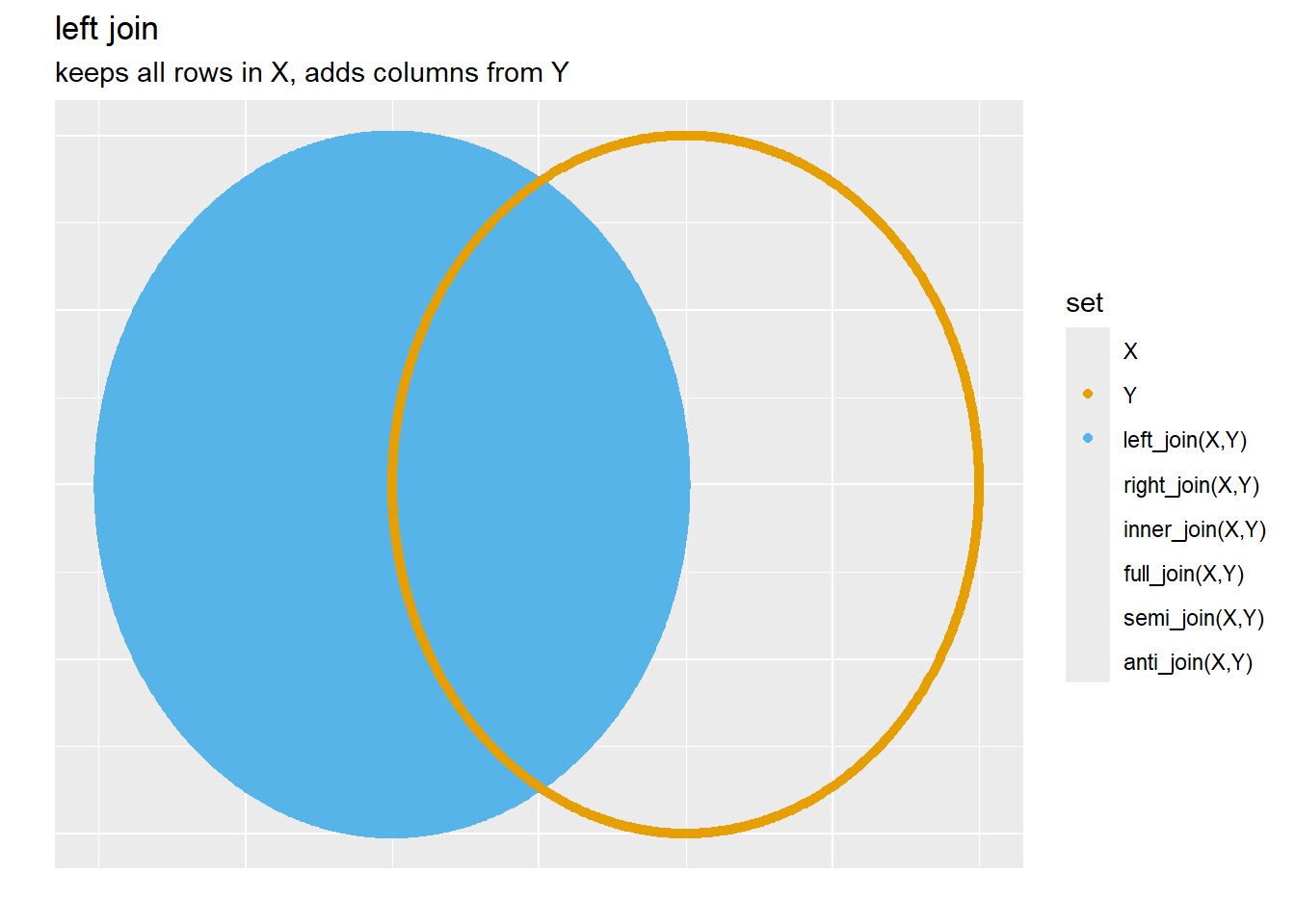
Let’s look at

Code

A %>%
  left_join(B) %>%
  knitr::kable(booktabs = TRUE, caption = 'A lef_join B')

Joining with `by = join_by(num)`

A lef_join B
num	char	Upper_char
1	a	NA
2	b	B
3	c	NA
4	d	D
5	e	NA
6	f	F

Note, above that every row in A (our x) is kept while adding the additional column from the B dataset, the columns are “joined” by the primary key (num)

Now, compare that to

Code

B %>%
  left_join(A)

Joining with `by = join_by(num)`

# A tibble: 3 × 3
    num Upper_char char 
  <dbl> <chr>      <chr>
1     2 B          b    
2     4 D          d    
3     6 F          f

Above, every record in B is kept however, the records in A that do not correspond to those in B by the primary key are not because B is our x in this instance.

3.6.1.1.2 Right Join

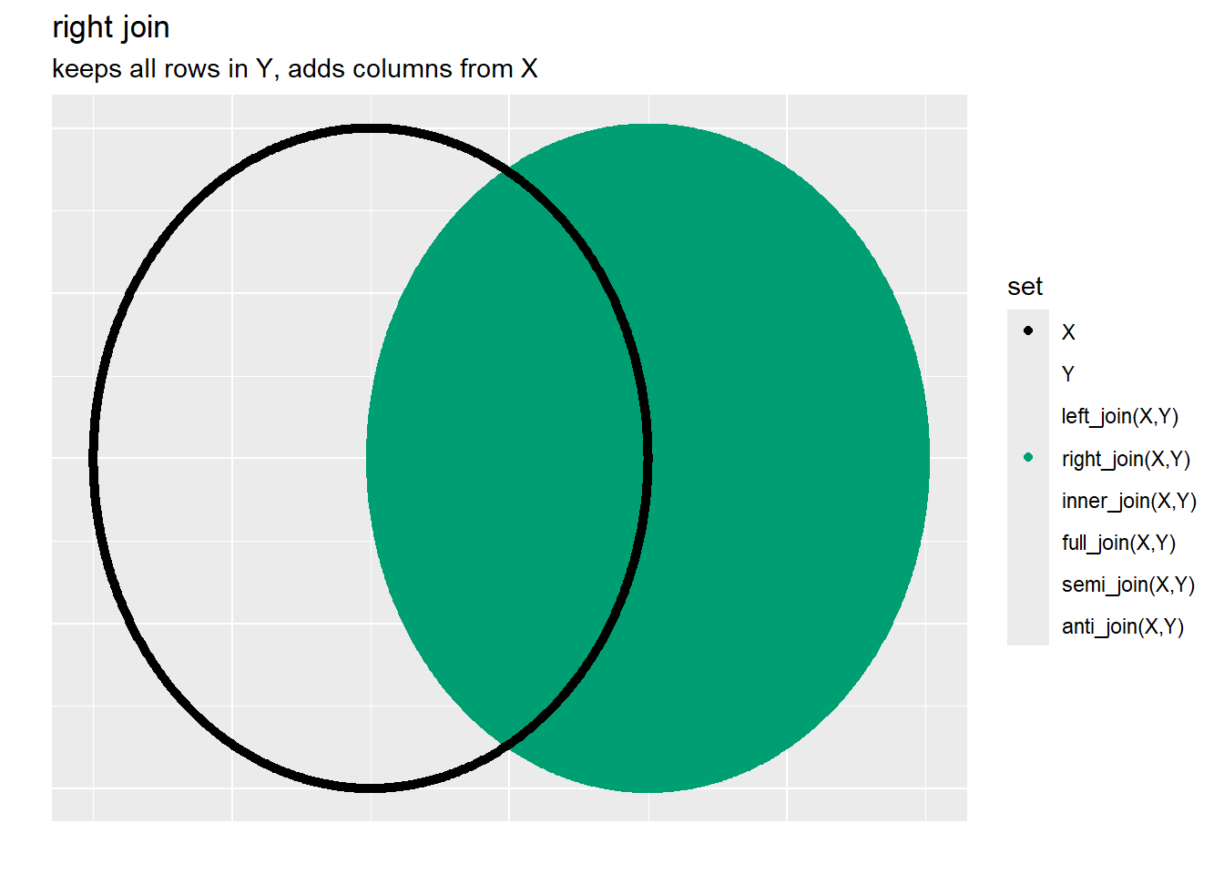
As another way to get to the same data in @ref(tab:A-left_join-B) would be

Code

B %>%
  right_join(A)

Joining with `by = join_by(num)`

# A tibble: 6 × 3
    num Upper_char char 
  <dbl> <chr>      <chr>
1     2 B          b    
2     4 D          d    
3     6 F          f    
4     1 <NA>       a    
5     3 <NA>       c    
6     5 <NA>       e

Note the results are out of order and the columns in B come first, however, could fix that with a simple arrange and select statements:

Code

B %>%
  right_join(A) %>%
  select(num, char, Upper_char) %>% 
  arrange(num) %>%
  knitr::kable(booktabs = TRUE, caption = 'B right_join A reformatted')

Joining with `by = join_by(num)`

B right_join A reformatted
num	char	Upper_char
1	a	NA
2	b	B
3	c	NA
4	d	D
5	e	NA
6	f	F

3.6.1.1.3 Inner Join

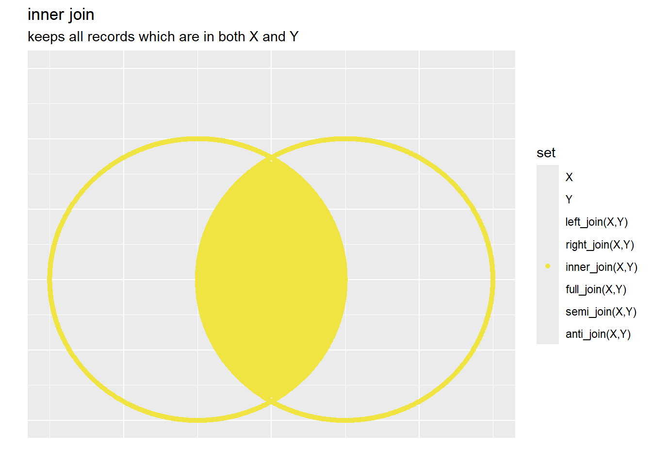
For inner joins, only records that have a primary keys that is in both x and y are maintained, the corresponding columns of y are still appended:

Code

A %>% 
  inner_join(B)

Joining with `by = join_by(num)`

# A tibble: 3 × 3
    num char  Upper_char
  <dbl> <chr> <chr>     
1     2 b     B         
2     4 d     D         
3     6 f     F

3.6.1.1.4 Semi Join

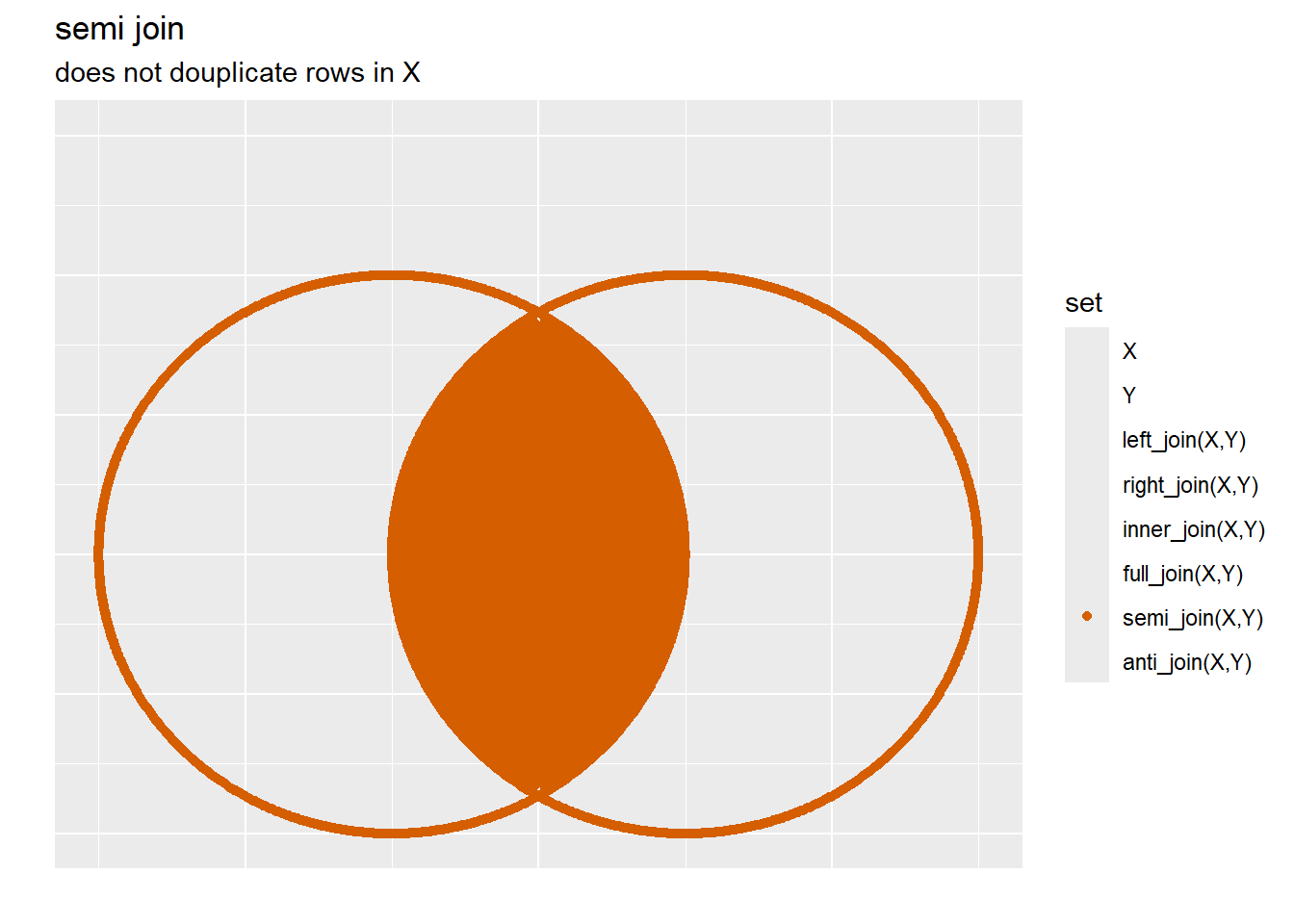
Similar to the inner_join above, the semi_join will keep only the records and columns contained within x so long as there is a corresponding record with a primary key in y:

Code

A %>%
  semi_join(B)

Joining with `by = join_by(num)`

# A tibble: 3 × 2
    num char 
  <int> <chr>
1     2 b    
2     4 d    
3     6 f

3.6.1.1.5 Anti Join

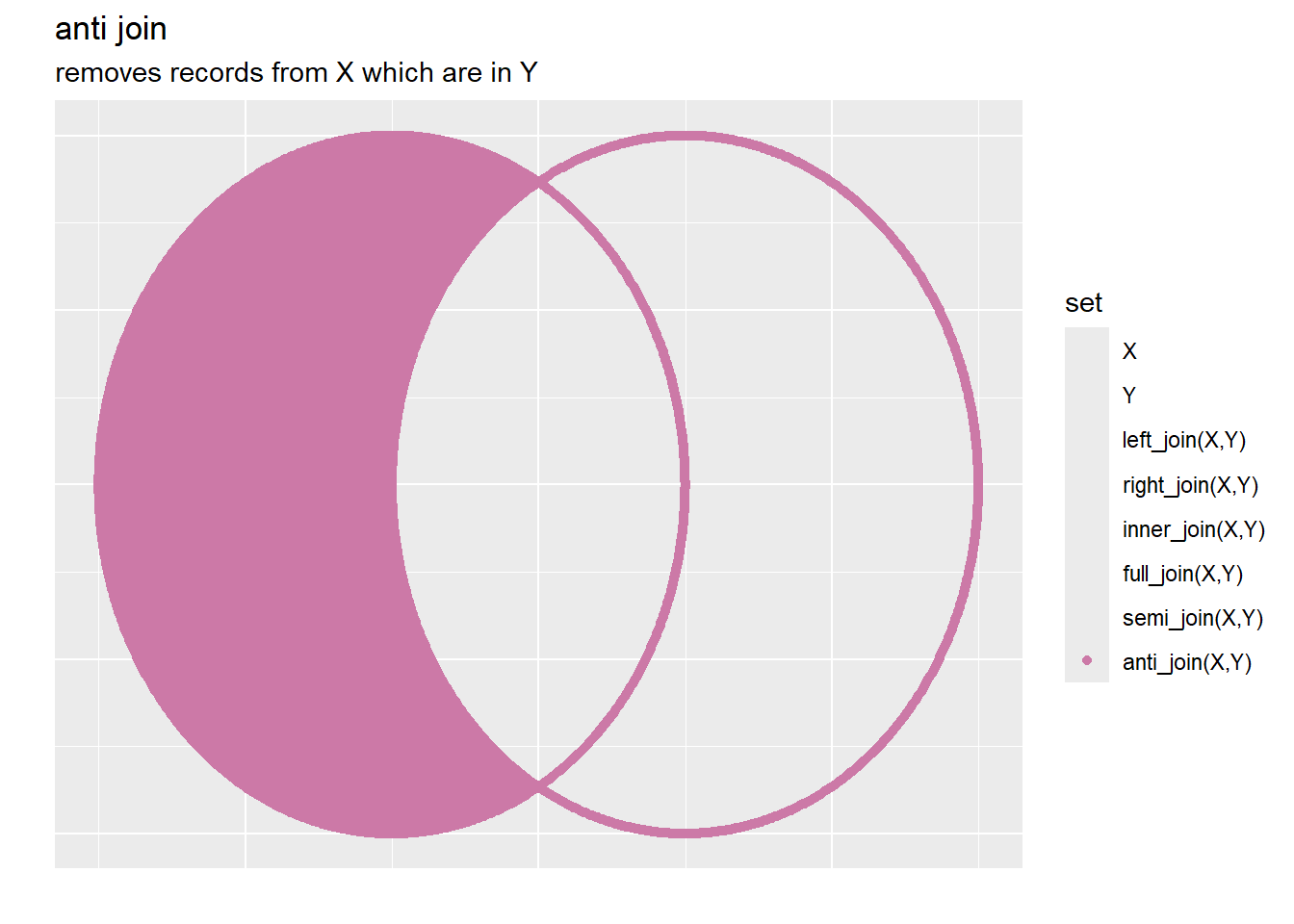
Anti Joins can be used to find all of the members of x not in y, (again this is done by the surggate key) note that no additional columns are added here, instead the records removed are the ones that are not in y.

Code

A %>% 
  anti_join(B)

Joining with `by = join_by(num)`

# A tibble: 3 × 2
    num char 
  <int> <chr>
1     1 a    
2     3 c    
3     5 e

3.6.1.1.6 Full Join

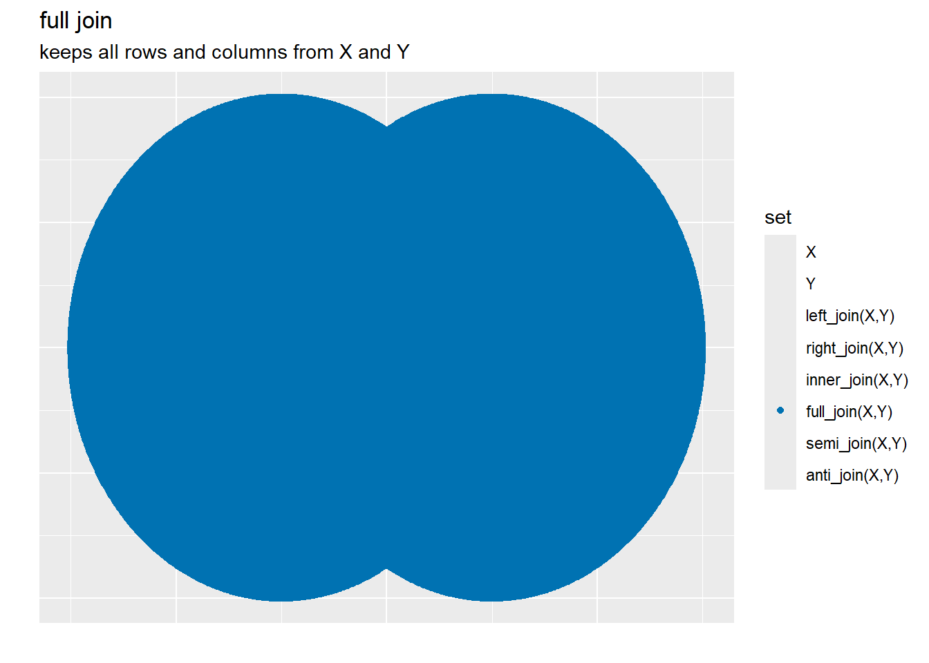
Full Joins will all keep all records and columns from both x and y, if there is a matching primary key in x and y then the columns of x and y are adjoined by the primary key:

Code

A_less_than_3 <- A %>%
  filter(num < 3)

A_less_than_3

# A tibble: 2 × 2
    num char 
  <int> <chr>
1     1 a    
2     2 b

Code

A_less_than_3 %>%
  full_join(B)

Joining with `by = join_by(num)`

# A tibble: 4 × 3
    num char  Upper_char
  <dbl> <chr> <chr>     
1     1 a     <NA>      
2     2 b     B         
3     4 <NA>  D         
4     6 <NA>  F

3.7 Left join Example

We will go over an example of left_join using the DIQ Table.

3.7.1 DIQ Table Example:

https://wwwn.cdc.gov/Nchs/Nhanes/2017-2018/DIQ_J.htm

Code

DIQ = tbl(NHANES_DB, "DIQ")
     
DIQ %>%
  glimpse()

Rows: ??
Columns: 81
Database: sqlite 3.46.0 [C:\Users\jkyle\Documents\GitHub\Jeff_R_Data_Wrangling\DATA\sql_db\NHANES.sqlite]
$ SEQN     <dbl> 1, 2, 3, 4, 5, 6, 7, 8, 9, 10, 11, 12, 13, 14, 15, 16, 17, 18…
$ DIQ010   <dbl> 2, 2, 2, 2, 2, 2, 2, 2, 2, 2, 2, 2, 1, 2, 2, 2, 2, 2, 2, 2, 2…
$ DIQ040G  <dbl> NA, NA, NA, NA, NA, NA, NA, NA, NA, NA, NA, NA, 1, NA, NA, NA…
$ DIQ040Q  <dbl> NA, NA, NA, NA, NA, NA, NA, NA, NA, NA, NA, NA, 67, NA, NA, N…
$ DIQ050   <dbl> NA, NA, 2, NA, 2, NA, 2, 2, 2, 2, 2, 2, 2, 2, NA, 2, NA, NA, …
$ DIQ060G  <dbl> NA, NA, NA, NA, NA, NA, NA, NA, NA, NA, NA, NA, NA, NA, NA, N…
$ DIQ060Q  <dbl> NA, NA, NA, NA, NA, NA, NA, NA, NA, NA, NA, NA, NA, NA, NA, N…
$ DIQ060U  <dbl> NA, NA, NA, NA, NA, NA, NA, NA, NA, NA, NA, NA, NA, NA, NA, N…
$ DIQ070   <dbl> NA, NA, NA, NA, NA, NA, NA, NA, NA, NA, NA, NA, 1, NA, NA, NA…
$ DIQ080   <dbl> NA, NA, NA, NA, NA, NA, NA, NA, NA, NA, NA, NA, 2, NA, NA, NA…
$ DIQ090   <dbl> NA, 2, NA, NA, 2, NA, 2, NA, NA, 1, NA, NA, 2, 2, NA, 2, NA, …
$ DIQ100   <dbl> NA, 2, NA, NA, 2, NA, 1, NA, NA, 2, NA, NA, 1, 2, NA, 2, NA, …
$ DIQ110   <dbl> NA, NA, NA, NA, NA, NA, 1, NA, NA, NA, NA, NA, 2, NA, NA, NA,…
$ DIQ120   <dbl> NA, 2, NA, NA, 2, NA, 2, NA, NA, 9, NA, NA, 2, 2, NA, 2, NA, …
$ DIQ130   <dbl> NA, NA, NA, NA, NA, NA, NA, NA, NA, NA, NA, NA, NA, NA, NA, N…
$ DIQ140   <dbl> NA, 2, NA, NA, 2, NA, 2, NA, NA, 2, NA, NA, 2, 2, NA, 2, NA, …
$ DIQ150   <dbl> NA, NA, NA, NA, NA, NA, NA, NA, NA, NA, NA, NA, NA, NA, NA, N…
$ yr_range <chr> "1999-2000", "1999-2000", "1999-2000", "1999-2000", "1999-200…
$ DID040G  <dbl> NA, NA, NA, NA, NA, NA, NA, NA, NA, NA, NA, NA, NA, NA, NA, N…
$ DID040Q  <dbl> NA, NA, NA, NA, NA, NA, NA, NA, NA, NA, NA, NA, NA, NA, NA, N…
$ DID060G  <dbl> NA, NA, NA, NA, NA, NA, NA, NA, NA, NA, NA, NA, NA, NA, NA, N…
$ DID060Q  <dbl> NA, NA, NA, NA, NA, NA, NA, NA, NA, NA, NA, NA, NA, NA, NA, N…
$ DID040   <dbl> NA, NA, NA, NA, NA, NA, NA, NA, NA, NA, NA, NA, NA, NA, NA, N…
$ DIQ220   <dbl> NA, NA, NA, NA, NA, NA, NA, NA, NA, NA, NA, NA, NA, NA, NA, N…
$ DIQ160   <dbl> NA, NA, NA, NA, NA, NA, NA, NA, NA, NA, NA, NA, NA, NA, NA, N…
$ DIQ170   <dbl> NA, NA, NA, NA, NA, NA, NA, NA, NA, NA, NA, NA, NA, NA, NA, N…
$ DIQ180   <dbl> NA, NA, NA, NA, NA, NA, NA, NA, NA, NA, NA, NA, NA, NA, NA, N…
$ DIQ190A  <dbl> NA, NA, NA, NA, NA, NA, NA, NA, NA, NA, NA, NA, NA, NA, NA, N…
$ DIQ190B  <dbl> NA, NA, NA, NA, NA, NA, NA, NA, NA, NA, NA, NA, NA, NA, NA, N…
$ DIQ190C  <dbl> NA, NA, NA, NA, NA, NA, NA, NA, NA, NA, NA, NA, NA, NA, NA, N…
$ DIQ200A  <dbl> NA, NA, NA, NA, NA, NA, NA, NA, NA, NA, NA, NA, NA, NA, NA, N…
$ DIQ200B  <dbl> NA, NA, NA, NA, NA, NA, NA, NA, NA, NA, NA, NA, NA, NA, NA, N…
$ DIQ200C  <dbl> NA, NA, NA, NA, NA, NA, NA, NA, NA, NA, NA, NA, NA, NA, NA, N…
$ DID060   <dbl> NA, NA, NA, NA, NA, NA, NA, NA, NA, NA, NA, NA, NA, NA, NA, N…
$ DID070   <dbl> NA, NA, NA, NA, NA, NA, NA, NA, NA, NA, NA, NA, NA, NA, NA, N…
$ DIQ230   <dbl> NA, NA, NA, NA, NA, NA, NA, NA, NA, NA, NA, NA, NA, NA, NA, N…
$ DIQ240   <dbl> NA, NA, NA, NA, NA, NA, NA, NA, NA, NA, NA, NA, NA, NA, NA, N…
$ DID250   <dbl> NA, NA, NA, NA, NA, NA, NA, NA, NA, NA, NA, NA, NA, NA, NA, N…
$ DID260   <dbl> NA, NA, NA, NA, NA, NA, NA, NA, NA, NA, NA, NA, NA, NA, NA, N…
$ DIQ260U  <dbl> NA, NA, NA, NA, NA, NA, NA, NA, NA, NA, NA, NA, NA, NA, NA, N…
$ DID270   <dbl> NA, NA, NA, NA, NA, NA, NA, NA, NA, NA, NA, NA, NA, NA, NA, N…
$ DIQ280   <dbl> NA, NA, NA, NA, NA, NA, NA, NA, NA, NA, NA, NA, NA, NA, NA, N…
$ DIQ290   <dbl> NA, NA, NA, NA, NA, NA, NA, NA, NA, NA, NA, NA, NA, NA, NA, N…
$ DIQ300S  <dbl> NA, NA, NA, NA, NA, NA, NA, NA, NA, NA, NA, NA, NA, NA, NA, N…
$ DIQ300D  <dbl> NA, NA, NA, NA, NA, NA, NA, NA, NA, NA, NA, NA, NA, NA, NA, N…
$ DID310S  <dbl> NA, NA, NA, NA, NA, NA, NA, NA, NA, NA, NA, NA, NA, NA, NA, N…
$ DID310D  <dbl> NA, NA, NA, NA, NA, NA, NA, NA, NA, NA, NA, NA, NA, NA, NA, N…
$ DID320   <dbl> NA, NA, NA, NA, NA, NA, NA, NA, NA, NA, NA, NA, NA, NA, NA, N…
$ DID330   <dbl> NA, NA, NA, NA, NA, NA, NA, NA, NA, NA, NA, NA, NA, NA, NA, N…
$ DID340   <dbl> NA, NA, NA, NA, NA, NA, NA, NA, NA, NA, NA, NA, NA, NA, NA, N…
$ DID350   <dbl> NA, NA, NA, NA, NA, NA, NA, NA, NA, NA, NA, NA, NA, NA, NA, N…
$ DIQ350U  <dbl> NA, NA, NA, NA, NA, NA, NA, NA, NA, NA, NA, NA, NA, NA, NA, N…
$ DIQ360   <dbl> NA, NA, NA, NA, NA, NA, NA, NA, NA, NA, NA, NA, NA, NA, NA, N…
$ DID341   <dbl> NA, NA, NA, NA, NA, NA, NA, NA, NA, NA, NA, NA, NA, NA, NA, N…
$ DIQ172   <dbl> NA, NA, NA, NA, NA, NA, NA, NA, NA, NA, NA, NA, NA, NA, NA, N…
$ DIQ175A  <dbl> NA, NA, NA, NA, NA, NA, NA, NA, NA, NA, NA, NA, NA, NA, NA, N…
$ DIQ175B  <dbl> NA, NA, NA, NA, NA, NA, NA, NA, NA, NA, NA, NA, NA, NA, NA, N…
$ DIQ175C  <dbl> NA, NA, NA, NA, NA, NA, NA, NA, NA, NA, NA, NA, NA, NA, NA, N…
$ DIQ175D  <dbl> NA, NA, NA, NA, NA, NA, NA, NA, NA, NA, NA, NA, NA, NA, NA, N…
$ DIQ175E  <dbl> NA, NA, NA, NA, NA, NA, NA, NA, NA, NA, NA, NA, NA, NA, NA, N…
$ DIQ175F  <dbl> NA, NA, NA, NA, NA, NA, NA, NA, NA, NA, NA, NA, NA, NA, NA, N…
$ DIQ175G  <dbl> NA, NA, NA, NA, NA, NA, NA, NA, NA, NA, NA, NA, NA, NA, NA, N…
$ DIQ175H  <dbl> NA, NA, NA, NA, NA, NA, NA, NA, NA, NA, NA, NA, NA, NA, NA, N…
$ DIQ175I  <dbl> NA, NA, NA, NA, NA, NA, NA, NA, NA, NA, NA, NA, NA, NA, NA, N…
$ DIQ175J  <dbl> NA, NA, NA, NA, NA, NA, NA, NA, NA, NA, NA, NA, NA, NA, NA, N…
$ DIQ175K  <dbl> NA, NA, NA, NA, NA, NA, NA, NA, NA, NA, NA, NA, NA, NA, NA, N…
$ DIQ175L  <dbl> NA, NA, NA, NA, NA, NA, NA, NA, NA, NA, NA, NA, NA, NA, NA, N…
$ DIQ175M  <dbl> NA, NA, NA, NA, NA, NA, NA, NA, NA, NA, NA, NA, NA, NA, NA, N…
$ DIQ175N  <dbl> NA, NA, NA, NA, NA, NA, NA, NA, NA, NA, NA, NA, NA, NA, NA, N…
$ DIQ175O  <dbl> NA, NA, NA, NA, NA, NA, NA, NA, NA, NA, NA, NA, NA, NA, NA, N…
$ DIQ175P  <dbl> NA, NA, NA, NA, NA, NA, NA, NA, NA, NA, NA, NA, NA, NA, NA, N…
$ DIQ175Q  <dbl> NA, NA, NA, NA, NA, NA, NA, NA, NA, NA, NA, NA, NA, NA, NA, N…
$ DIQ175R  <dbl> NA, NA, NA, NA, NA, NA, NA, NA, NA, NA, NA, NA, NA, NA, NA, N…
$ DIQ175S  <dbl> NA, NA, NA, NA, NA, NA, NA, NA, NA, NA, NA, NA, NA, NA, NA, N…
$ DIQ175T  <dbl> NA, NA, NA, NA, NA, NA, NA, NA, NA, NA, NA, NA, NA, NA, NA, N…
$ DIQ175U  <dbl> NA, NA, NA, NA, NA, NA, NA, NA, NA, NA, NA, NA, NA, NA, NA, N…
$ DIQ175V  <dbl> NA, NA, NA, NA, NA, NA, NA, NA, NA, NA, NA, NA, NA, NA, NA, N…
$ DIQ175W  <dbl> NA, NA, NA, NA, NA, NA, NA, NA, NA, NA, NA, NA, NA, NA, NA, N…
$ DIQ275   <dbl> NA, NA, NA, NA, NA, NA, NA, NA, NA, NA, NA, NA, NA, NA, NA, N…
$ DIQ291   <dbl> NA, NA, NA, NA, NA, NA, NA, NA, NA, NA, NA, NA, NA, NA, NA, N…
$ DIQ175X  <dbl> NA, NA, NA, NA, NA, NA, NA, NA, NA, NA, NA, NA, NA, NA, NA, N…

Code

DEMO.DIQ <- DEMO %>%
  left_join(DIQ)

Joining with `by = join_by(SEQN, yr_range)`

One thing to notice in the eaxmples above is that we did not specify by in left_join - R searched both tables for column names and made an assumption. This can be both beneficial and dangerous if users are unfamiliar with the data.

If we wanted to be more explicit or exhibit a different level of control we can join by a specific column:

Code

DEMO.DIQ_by_yr_range <- DEMO %>%
  left_join(DIQ, by = c("yr_range"="yr_range"))

DEMO.DIQ_by_yr_range %>%
  select(contains('SEQN')) %>%
  colnames()

[1] "SEQN.x" "SEQN.y"

You can see in this case R will produce two columns in the output labeled with .x and .y buy default. At times, it might be advantageous to control that as well, it can be accomplished with the suffix parameter:

Code

DEMO.DIQ_by_yr_range <- DEMO %>%
  left_join(DIQ, 
            by = c("yr_range"="yr_range"),
            suffix = c("_DEMO","_DIQ"))

DEMO.DIQ_by_yr_range %>%
  select(contains('SEQN')) %>%
  colnames()

[1] "SEQN_DEMO" "SEQN_DIQ"

Code

DEMO.DIQ_by_SEQN <- DEMO %>%
  left_join(DIQ, 
            by = c("SEQN"="SEQN"),
            suffix = c("_DEMO","_DIQ"))

DEMO.DIQ_by_SEQN %>%
  select(contains('yr_range')) %>%
  colnames()

[1] "yr_range_DEMO" "yr_range_DIQ"

Code

DEMO.DIQ_by_SEQN_yr_range <- DEMO %>%
      left_join(DIQ, by=c("SEQN"="SEQN", 'yr_range'='yr_range'))

3.7.2 Question

Which of the above would you use for what situation? Why?

3.8 NHANES Table Helpers

3.8.1 `NHANES_table_helper`

To get started learning how to write your own helper functions you can review this example here. We provide the function NHANES_table_helper with a Table_Name and it will return for us a text url link url_link:

Code

NHANES_table_helper <- function(Table_Name){
  url_link <- paste0('https://wwwn.cdc.gov/Nchs/Nhanes/2017-2018/',Table_Name,'_J.htm')
  return(url_link)
}

3.8.1.1 Test out function:

Code

NHANES_table_helper('DR1TOT')

Code

NHANES_table_helper(NHANES_Tables[2])

3.8.2 `Open_NHANES_table_help`

Code

Open_NHANES_table_help <- function(Table_Name){
  
  if(Table_Name %in% NHANES_Tables){
    return(browseURL(NHANES_table_helper(Table_Name)))} 
  else {
    ln1 <- paste0("ERROR : ", Table_Name, " is not a valid table name! \n")
    ln2 <- 'Please Choose one of : \n'
    ln3 <- NHANES_Tables
    cat(ln1)
    cat(ln2)
    cat(ln3)
  }
}

Code

Open_NHANES_table_help('FROG')

Code

Open_NHANES_table_help('DEMO')

3.1 Connect to SQLite database

3.2 List of tables

3.3 Demographics Table

3.4 dplyr vocabulary

3.5 dplyr %>% SQL

3.6 JOINS

3.6.1 DPLYR JOINS

3.6.1.1 Quick Examples

3.6.1.1.1 Left Join

3.6.1.1.2 Right Join

3.6.1.1.3 Inner Join

3.6.1.1.4 Semi Join

3.6.1.1.5 Anti Join

3.6.1.1.6 Full Join

3.7 Left join Example

3.7.1 DIQ Table Example:

3.7.2 Question

3.8 NHANES Table Helpers

3.8.1 NHANES_table_helper

3.8.1.1 Test out function:

3.8.2 Open_NHANES_table_help

3.4 `dplyr` vocabulary

3.5 `dplyr` `%>%` SQL

3.8.1 `NHANES_table_helper`

3.8.2 `Open_NHANES_table_help`